Reduce WER with 3–5 Diverse ASR Models for Developers

Reduce WER with 3–5 Diverse ASR Models for Developers

Running audio through several ASR models and merging the results with recognizer output voting error reduction (ROVER), confidence-based selection, or LLM reconciliation reduces word error rate beyond what any single model achieves alone. Accuracy-first pipelines should run three to five diverse models in parallel and fuse with ROVER; cost- or latency-constrained pipelines should route per segment to whichever model reports the highest calibrated confidence. Model diversity and per-segment resolution, not the number of models, drive most of the gain.

TL;DR:

• Combining three to five diverse ASR models using ROVER generally captures most of the accuracy improvements while keeping costs manageable.
• Confidence-based selection requires well-calibrated scores and offers a low-cost, fast alternative to full fusion, especially when model confidence is reliable.
• LLM reconciliation improves accuracy in ambiguous regions but adds latency and cost, making it suitable only for complex or uncertain segments.
• Building a robust pipeline involves audio normalization, parallel model invocation with timeouts, structured result collection, and careful speaker-label mapping before fusion.
• Running shadow tests on representative data allows calibration of confidence thresholds, while continuous metric tracking ensures stable deployment and quick detection of issues.

Table of Contents

• Fusion Strategies: ROVER, Confidence Selection, and LLM Reconciliation
• How to Build an ASR Model Combination Pipeline
• Latency, Cost, and Accuracy Trade-Offs
• Deployment Checklist: QA, Metrics, and Common Pitfalls
• How OpenTranscription Fits This Playbook
• Start Benchmarking a Diverse Model Set Today
• Sources
• FAQ

Fusion Strategies: ROVER, Confidence Selection, and LLM Reconciliation

Three approaches dominate practitioner use, and each fits a different combination of available data and latency budget.

ROVER works by aligning multiple hypotheses with dynamic programming (DP), building a word transition network (WTN) or confusion network, and picking the consensus word through majority or weighted voting. NIST’s original ROVER research established this as the reference algorithm for hypothesis fusion, and it still performs best when at least one model exposes calibrated confidence scores or decoder-level detail. When those scores are missing or unreliable, quality estimation (QE) steps in. QE-informed ROVER ranks hypotheses at the segment level instead of relying on raw confidence, and tests on black-box systems showed absolute word error rate improvements between 0.5% and 7.3% over standard ROVER, according to research on automatic quality estimation for ASR combination.

Confidence-based selection skips full fusion entirely. You run the candidate models in parallel and, for every segment, keep the output from whichever model reports the highest confidence. Interspeech research on confidence-based ensembles found this approach can match or beat dedicated adaptation or language-identification blocks, provided the confidence scores are well calibrated across models. Entropy-based confidence measures help correct for models that report inflated certainty.

LLM reconciliation handles the cases voting can’t resolve cleanly. Feeding the conflicting regions, or full competing hypotheses, into a text-based or speech-aware LLM lets the model use context and world knowledge to pick a winner. Research on textual and speechLLM postprocessing for multi-ASR pipelines has shown this method also generates stronger pseudo-labels than rule-based cascades, which matters if you’re building training data from ensemble output.

A few operational notes worth keeping in view:

• ROVER needs alignment infrastructure but no model internals beyond word timestamps.
• Confidence selection is cheap to run but demands calibration work up front.
• LLM reconciliation adds latency and cost, so reserve it for ambiguous regions rather than full transcripts.
• When lattice- or frame-level access is available, rescoring at that finer grain typically beats hypothesis-level voting, though it requires decoder internals most black-box APIs don’t expose.

How to Build an ASR Model Combination Pipeline

A combination pipeline has six stages: audio preprocessing, parallel or staged model execution, result collection, alignment, speaker-label mapping, and fusion, followed by an optional LLM postprocess step. Each stage feeds structured output, including model provenance and per-hypothesis confidence, into the next.

1. Normalize the audio. Resample, apply consistent gain, and pick a chunking strategy. Sliding windows suit streaming; fixed segments suit batch jobs where you control the file boundaries.
2. Invoke models with per-model timeouts. A slow or hung backend shouldn’t stall the whole pipeline. Open-source implementations such as ovos-stt-plugin-rover demonstrate parallel backend execution with per-backend timeouts feeding directly into ROVER merging.
3. Collect transcripts, timestamps, and confidences. Store these with a record of which model produced them.
4. Build the word transition network. Use DP alignment with roughly 100 millisecond time bins, as recommended in the meeting-recognition MOVER research. When word-level timing is missing, approximate it with pseudo-word timing proportional to character counts or run forced alignment first.
5. Vote or select. Apply weighted voting across the WTN, or select the single highest-confidence hypothesis per segment if you’re running the lighter-weight pattern.
6. Merge timestamps and speaker labels. Map diarization output from each model onto a common speaker set before finalizing the transcript. The same MOVER research extends ROVER specifically to handle systems that produced different diarization boundaries.

For streaming deployments, implement incremental WTN construction with a flush policy: fuse every few seconds or at detected sentence boundaries rather than waiting for the full utterance, which keeps end-to-end latency predictable. Whatever the failure mode, degrade gracefully. If one model times out or errors, fall back to single-model output rather than blocking the request, and always tag the final transcript with which models actually contributed.

Pro Tip: Log model provenance on every word, not just every segment. When an audit or a customer complaint requires tracing an error back to its source model, segment-level provenance is often too coarse to be useful.

Latency, Cost, and Accuracy Trade-Offs

Parallel execution latency tracks the slowest model in the set, not the sum of all of them. Running four models simultaneously costs you roughly max(latency) across those models rather than their total, which is the entire appeal of the parallel pattern over sequential fallback chains. Staged or selective execution flips that trade: you add a small decision-latency overhead deciding which model to trust, but you can skip running the others entirely once one model’s confidence clears your threshold.

Cost follows a different curve. Running N models concurrently means paying for N models’ worth of processing time on every request, since per-second billing scales linearly with runtime across all active models. Selective execution, where you only escalate to a second or third model when the first reports low confidence, often cuts cost substantially because most audio doesn’t need the full ensemble.

Model diversity is the lever that actually moves accuracy, more than model count does. Mixing architectures, end-to-end transformer transducers alongside hybrid Kaldi-style decoders, with different training data, captures errors that near-identical models share and vote past. Research combining hybrid and end-to-end speech recognition reported word error rate reduction of roughly 14% in some tested configurations when diversity and calibration were both handled carefully.

• A small number of diverse models tend to capture most of the available ensemble gain without ballooning compute or complexity.
• Adding a sixth or seventh model that’s architecturally similar to ones already in the set rarely moves the needle.
• If your candidate models are black boxes with poorly calibrated confidence, apply QE ranking or build a small calibration dataset before trusting raw scores in a weighted vote.

A practitioner benchmark worth internalizing: multi-model ensemble notes from the field suggest running three to five diverse models captures most of the available accuracy improvement, with diminishing returns beyond that range as compute cost keeps climbing.

Deployment Checklist: QA, Metrics, and Common Pitfalls

Before any combined pipeline reaches production, run it against a representative corpus in shadow mode, measuring segment-level WER and word error rate reduction (WERR) against each standalone model. That shadow run is also where you calibrate confidence thresholds, since production traffic almost always differs from whatever set you tuned on originally.

Once live, track four metrics continuously:

1. Latency at P50 and P95, not just average, since tail latency is what breaks SLAs.
2. Ensemble disagreement rate, the share of segments where models diverge, as a leading indicator of drift or a misbehaving backend.
3. Cost per audio second, tracked separately for parallel and selective paths.
4. The calibration curve, plotting reported confidence against actual accuracy, rechecked periodically since drift degrades calibration silently.

Set alerts on sudden jumps in disagreement rate, model outages, or latency regressions, and keep a sample of misaligned segments on hand for debugging speaker-label mapping, which is where research on diarization consistency in ASR combination identifies the most common integration bug.

The three pitfalls that recur most often: skipping speaker-label alignment before fusion, trusting raw confidence scores from a model that’s simply overconfident by design, and scaling to more parallel models without recalculating the cost curve.

Pro Tip: Run your calibration checks on a rolling window, not a one-time offline dataset. A model that was well calibrated at launch can drift as its provider updates the underlying weights.

How OpenTranscription Fits This Playbook

Everything in this guide assumes you can actually get multiple ASR outputs into one pipeline without building a separate integration for each provider. That’s the specific problem OpenTranscription’s API is built to remove: it gives you access to more than 30 transcription models through one interface, with structured transcripts, word-level confidence scores, real-time streaming, speaker identification, and support for more than 105 languages.

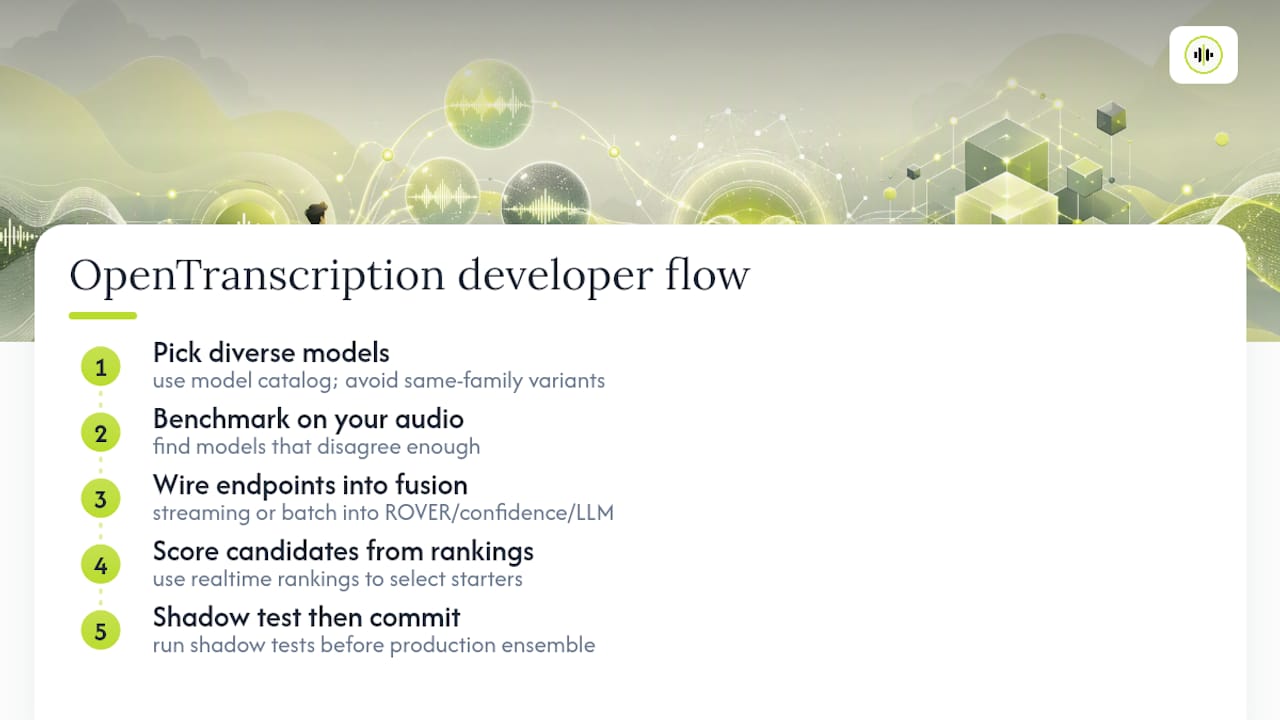
A typical developer flow starts in the model catalog, where you pick two or three architecturally distinct models rather than three variations on the same base transformer. From there, benchmarking jobs on your own representative audio tell you which models actually disagree often enough to be worth combining, versus which ones are redundant. Then you wire the platform’s streaming or batch endpoints directly into the fusion architecture described above, ROVER, confidence selection, or LLM reconciliation, without maintaining separate SDKs per vendor.

If you’re deciding where to start, pull a first candidate set from the realtime rankings and run shadow tests before committing to a production ensemble.

— Benjamin

Start Benchmarking a Diverse Model Set Today

Building the ensemble described in this guide gets a lot faster when you’re not manually stitching together API contracts for every provider. OpenTranscription gives you one integration point across many transcription models, with transparent per-second billing and no subscription commitment, so testing a three-model or five-model set costs exactly what you use and nothing more.

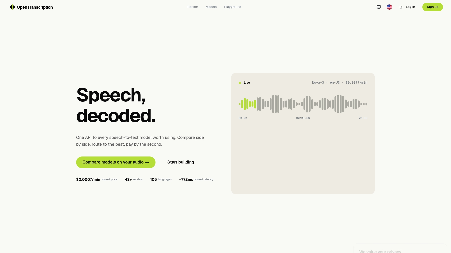
Start by browsing the transcription model catalog to identify candidates with genuinely different architectures, then run them side by side through the comparison and benchmarking tools against your own audio. If latency is your binding constraint, check the realtime model rankings before locking in your ensemble. Every job returns structured output with confidence scores and model provenance built in, so the alignment and fusion work described earlier in this guide has clean data to work from instead of ad hoc logging. Grab an API key and run a shadow test against your own corpus before deciding which combination pattern fits your SLA.

Sources

• NIST: Post-processing system yields reduced word error rates: Recognizer Output Voting Error Reduction (ROVER)
• Confidence-based ensembles of end-to-end speech recognition models (Interspeech 2023)

FAQ

What Is ROVER in ASR Model Combination?

ROVER (Recognizer Output Voting Error Reduction) aligns multiple ASR transcripts into a word transition network and selects the winning word at each position through majority or weighted voting, a method originally described by NIST.

How Many Models Should I Combine for Best Results?

Three to five architecturally diverse models typically capture most of the available accuracy gain, according to practitioner ensemble notes, with additional similar models adding cost more than accuracy.

Does Combining ASR Models Increase Latency?

Running models in parallel keeps latency close to your slowest model rather than the sum of all of them, but staged or selective execution adds a small decision step while often lowering total cost.

What Is Quality Estimation in ASR Fusion?

Quality estimation (QE) ranks competing ASR hypotheses at the segment level when decoder confidence isn’t available, and QE-informed ROVER has shown absolute WER improvements of 0.5% to 7.3% over standard voting in tested scenarios.

Can I Combine Models With Different Speaker Diarization Output?

Yes, but you need to map speaker labels across systems before fusion. The MOVER method extends ROVER specifically to reconcile differing diarization boundaries in meeting audio.

How Do I Test an Ensemble Before Deploying It?

Run a shadow test against a representative audio corpus, measure segment-level WER against each standalone model, and calibrate confidence thresholds before switching production traffic over. OpenTranscription’s model comparison tools support this kind of side-by-side evaluation on your own audio.