

Cut WER and Cost in 90 Minutes: ASR Model Selection by Segment Routing
The most reliable way to cut both word error rate and inference cost is to stop treating model selection as a single, static choice and instead route each audio segment to the smallest model that can handle it. Recent experiments confirm this: a lightweight decision module that dynamically assigns segments across a pool of ASR systems delivered a relative word error rate (WER) reduction alongside significantly lower cost and faster processing versus a single-best baseline, as documented in AutoMode-ASR. The rest of this guide covers the features, evaluation protocol, and implementation steps behind that result.
TL;DR:
- Routing audio segments to the smallest capable model reduces overall word error rate and inference costs, as confirmed by recent experiments.
- Effective decision modules should prioritize cheap features like signal-to-noise ratio and voice activity detection before considering high-dimensional embeddings.
- Evaluating routing systems with an oracle baseline helps determine the true potential of segment-level model selection before committing to a production classifier.
- Building a reliable pipeline involves six steps, including segmentation, feature extraction, classifier training, inference, rescoring, and telemetry, tailored to deployment context.
- Testing model performance on your actual audio and using platform tools like OpenTranscription accelerates efficient experimentation and precise model selection.
Table of Contents
- What Is Model Selection in ASR, and Why Does Routing Beat a Single Model?
- Which Signals Should Feed the Decision Module?
- How Do You Evaluate and Benchmark a Selection System?
- How Should You Handle Data Selection for Low-Resource Languages?
- What Does a Reproducible Model-Selection Workflow Look Like?
- What Are the Engineering Trade-Offs in Cost, Latency, and Licensing?
- How OpenTranscription Accelerates Model-Selection Experiments
- How Do You Handle Domain Mismatch and Noise Robustness?
- How Does Model Selection Integrate With End-to-End ASR Pipelines?
- What Do Real-World Case Studies Show About Model-Selection Impact?
- How Do You Reduce Feature Dimensionality for Routing Decisions?
- What the Research Actually Supports, and What It Doesn’t
- Prototype Your Routing Strategy in an Afternoon
- Sources
- FAQ
What Is Model Selection in ASR, and Why Does Routing Beat a Single Model?
Model selection in automatic speech recognition refers to the process of choosing which recognition system, or combination of systems, handles a given piece of audio, rather than committing an entire pipeline to one architecture regardless of acoustic conditions. The dominant paradigms have converged on three related but distinct strategies.
Dynamic, segment-level routing is the approach behind AutoMode-ASR, which trains a decision module (typically a binary classifier or a small ensemble) to predict, per segment, whether a specialized model or a general-purpose model will produce the lower-error transcript. The module runs on audio and transcript-derived features, then routes accordingly, rather than running every candidate model on every segment.
Unsupervised accent identification (AID) based selection takes a different angle: instead of predicting WER directly, the system first classifies the speaker’s accent or dialect cluster, then routes to a model fine-tuned for that cluster. This matters because AID-based routing frequently outperforms blind speaker adaptation when labeled adaptation data is scarce, since adaptation requires per-speaker fine-tuning data that most production pipelines never have in useful volume.
Sample-dependent small-versus-large routing, demonstrated in Whisper-focused research, reserves the largest model for audio flagged as acoustically “hard” and defaults everything else to a smaller, cheaper model. This sample-dependent routing work shows substantial compute savings with only modest accuracy trade-offs, because most conversational audio is not actually hard.
Each approach fails differently:
- Dynamic routing degrades when the decision module is trained on data that does not reflect production noise conditions.
- AID-based selection struggles with code-switching speakers or accent clusters absent from training data.
- Sample-dependent routing can misclassify moderately noisy segments as “easy,” under-provisioning the model and inflating WER on exactly the content where accuracy matters most.
Which Signals Should Feed the Decision Module?
The decision module is only as good as its inputs, and not every feature is worth its extraction cost. Prioritize signals in this order:
- Self-supervised audio embeddings (wav2vec2, XLSR) capture acoustic and phonetic structure without requiring labels, and they generalize across languages better than hand-engineered features, making them the strongest default for cross-lingual routing.
- Lightweight ASR-derived transcript features, including n-gram density and out-of-vocabulary (OOV) rate, come from running a compact, fast ASR model as a temporary pass, a design pattern AutoMode-ASR uses specifically to keep decision-time overhead low.
- Signal statistics, such as signal-to-noise ratio (SNR), voice activity detection (VAD) density, and reverberation proxies, are cheap to compute and useful as a first filter before investing in embeddings.
- Quality estimation (QE) and confidence scores rescore candidate outputs after an initial pass; adding a QE rescoring stage to AutoMode-style pipelines produced further WER gains at limited added cost.
Pro Tip: Start with SNR and VAD density alone. If your decision module already separates easy from hard segments well on those two cheap signals, you may not need embeddings at all for a first production pass.
How Do You Evaluate and Benchmark a Selection System?
Word error rate (WER) remains the primary accuracy metric, with character error rate (CER) and named-entity error metrics layered on for domains like medical or legal transcription where a single misrecognized entity carries outsized consequences.
Efficiency needs equal billing. Track:
- RTFx (real-time factor, inverse), which the Open ASR Leaderboard’s standardized benchmarking across 86 systems and 12 datasets uses to expose the core trade-off: Conformer plus transformer decoder architectures post the strongest average WER, while CTC and TDT decoders deliver far better throughput.
- Cost per GPU-second and per audio-hour, which turns raw accuracy gains into a defensible budget line.
- Latency budget per segment, particularly for streaming deployments where the routing decision itself must not become the bottleneck.
Design your test set deliberately rather than relying on a generic benchmark split: hold out noisy segments, accented speech, and long-form audio separately so you can see where routing helps and where it doesn’t. Build an oracle baseline (perfect hindsight selection) and a pivot baseline (single best-performing model) to bound your decision module’s realistic ceiling and floor.
For ablations, isolate feature importance, test QE rescoring with and without it, and vary sample-weighting during decision-module training to see which change moved the needle. The relative WER reduction cited earlier came from exactly this kind of structured comparison against a single-best baseline, not from an isolated demo run.
How Should You Handle Data Selection for Low-Resource Languages?
Under-resourced languages punish a common assumption: that picking the highest-ranked global architecture is the safest bet. Research on model selection guidance for under-resourced languages found the opposite. No single architecture consistently dominates across low-resource settings, and data quality plus selection strategy typically matters more than architecture choice, according to ACL/Computel research.
- Submodular selection methods build small, representative training corpora that improve language-model quality using less data than random sampling, a result confirmed in submodular data selection research from the University of Washington.
- Synthetic TTS augmentation helps when your target domain lacks acoustic diversity, but it introduces distribution mismatch risk when the synthetic voice characteristics diverge from real speaker populations, so validate on held-out real audio before trusting augmented gains.
- Small-sample AID-based selection frequently beats blind adaptation for a new language variant. Run a quick per-language test with AID routing before committing engineering time to full fine-tuning.
What Does a Reproducible Model-Selection Workflow Look Like?
A working pipeline breaks into six stages, and skipping any one of them is the most common reason teams see disappointing routing gains in production despite promising offline numbers.
- Segmentation and VAD. Split audio into segments using voice activity detection, tuned to your typical utterance length rather than a generic default.
- Feature extraction. Run the compact ASR pass, compute signal statistics, and pull audio embeddings, all before any full-size model touches the segment.
- Routing classifier training. Train the decision module using delta-WER against a pivot system as the label, rather than absolute WER, since delta-WER highlights exactly where a non-default model meaningfully helps rather than diluting the signal with segments where every model performs similarly.
- Selected inference. Route each segment to its assigned model based on the classifier’s prediction.
- QE rescoring. Apply a quality-estimation pass on ambiguous or borderline routing decisions to catch cases the classifier is unsure about.
- Telemetry. Log per-segment WER estimates, routing decisions, and latency for every production call.
Deployment patterns diverge by use case. Streaming systems need asynchronous routing decisions and compact feature extractors so the decision itself doesn’t add perceptible delay. Batch systems have more latitude and can afford a heavier decision module if it improves accuracy further.
Pro Tip: Run an offline oracle experiment first, using perfect hindsight to pick the best model per segment. That gives you the theoretical upper bound before you invest in a real classifier, so you know exactly how much headroom is left to capture.
Monitoring in production should track per-slice WER (broken out by noise level, accent cluster, and length), drift alerts when a slice’s error rate creeps upward, and automated rollback thresholds that revert to the pivot model if a routing update degrades a monitored slice beyond a set tolerance.
What Are the Engineering Trade-Offs in Cost, Latency, and Licensing?
Return on investment for a decision module comes down to a simple comparison: decision-module compute cost against the inference savings it generates. If the classifier itself is expensive to run, you can erase the gains it’s supposed to capture, which is why AutoMode-ASR’s design deliberately keeps the feature-extraction pass lightweight.
- Latency budgeting matters most for streaming and voice-agent deployments, where the routing decision must fit inside the conversational turn-taking window rather than adding a visible pause; the voice AI latency engineering guide covers how an 800ms conversational budget constrains architecture choices.
- License and attribution checklists deserve a pass before adoption, since CC-BY obligations can become a blocker in commercial pipelines where attribution requirements conflict with product packaging.
- Privacy handling for intermediate transcripts and feature telemetry needs the same scrutiny as final outputs, since a temporary transcript pass still contains sensitive content even if it’s discarded after routing.
- When top models differ by less than one WER point, license terms, language coverage, and streaming support usually decide the procurement call more than the leaderboard rank itself.
How OpenTranscription Accelerates Model-Selection Experiments
Testing the routing strategies above traditionally means standing up infrastructure for a dozen or more ASR systems before you can run a single comparison. OpenTranscription’s model catalog and realtime ranking tool shortcut that step by exposing benchmark data across 40+ transcription models, spanning 105+ languages, cost, and speed metrics, in one interface.
A practical experiment: upload a representative 10 to 20 minute audio sample through the platform, run per-model WER and cost comparisons, then use the resulting metrics as ground truth for training your own pivot classifier. Because the platform reports word-level confidence scores alongside each transcript, those scores double as an early quality-estimation feature for your decision module before you build a dedicated QE model.
How Do You Handle Domain Mismatch and Noise Robustness?
Domain mismatch is the quiet killer of otherwise well-tuned selection systems. A decision module trained on clean, single-speaker call center audio will misroute badly on multi-speaker meeting recordings or far-field smart-speaker audio, because the feature distributions it learned to interpret no longer match what it sees in production.
The fix starts with test-set design, not model architecture. Build validation slices that mirror your actual deployment conditions: reverberant rooms, overlapping speech, background music, and compressed telephony audio, rather than relying on a single clean benchmark split. If your production traffic includes accented speech underrepresented in training, treat that as its own slice with its own WER tracking, not an average blended into overall numbers where it can hide.
Noise robustness testing benefits from injecting realistic noise profiles, room impulse responses, and codec artifacts into a held-out clean set, rather than only evaluating on naturally noisy recordings, because synthetic noise injection lets you isolate exactly which noise types degrade which models. A decision module that routes well on lab-quality audio can still fail when SNR drops below the range it was trained on, so extend your training distribution to cover the SNR floor you expect in production, not just the median case.
Cross-domain generalization also depends on how the module’s features were extracted. Self-supervised audio embeddings tend to transfer across domains better than transcript-derived features like OOV rate, because vocabulary shifts far more between domains than acoustic structure does. When domain mismatch is severe, weight embedding-based features more heavily in the classifier and treat transcript-derived signals as a secondary check rather than a primary input.
How Does Model Selection Integrate With End-to-End ASR Pipelines?
A routing layer only helps if it slots cleanly into the pipeline stages that come before and after it. Positioned correctly, the decision module sits between voice activity detection and the final inference call, consuming segment boundaries as input and emitting a model assignment as output, without requiring changes to upstream audio capture or downstream transcript formatting.
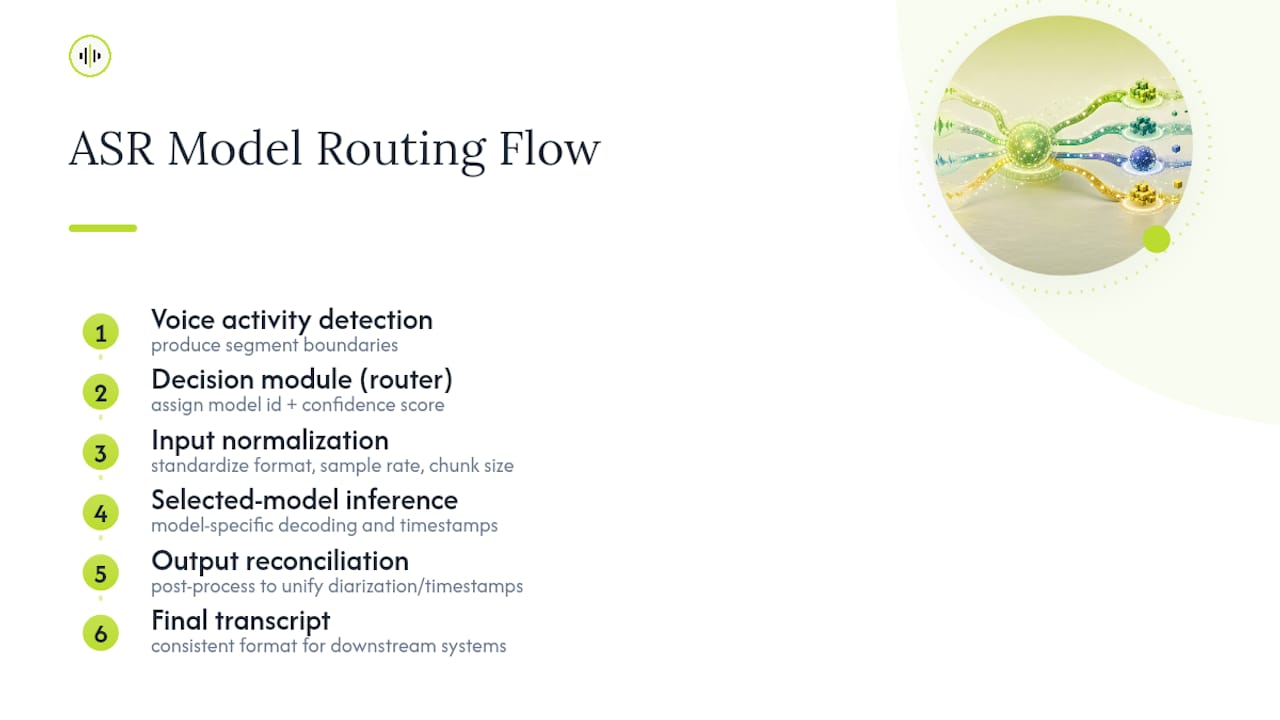
The integration challenge usually shows up at the interface boundaries. Different ASR models expect different audio formats, sample rates, and chunk sizes, so the routing layer needs a normalization step that standardizes input before dispatch, otherwise you’re debugging format mismatches instead of measuring routing accuracy. Output formatting matters just as much: if downstream systems expect consistent timestamp granularity or speaker diarization tags, the selected model must support those features, or the pipeline needs a post-processing pass to reconcile differences between models’ native output formats.
For streaming pipelines specifically, integration means the decision module’s latency has to fit inside the same real-time constraint as the ASR models themselves. A streaming-focused evaluation approach favors compact encoder features with sliding-window embeddings precisely because chunk size and perceived turn-taking latency matter more for voice-agent user experience than batch WER numbers ever will. Batch pipelines have more room to run a heavier decision module, since a few hundred milliseconds of added latency per segment rarely matters when the job runs asynchronously overnight.
The cleanest integrations treat the router as a pluggable component with a stable interface contract: given a segment and its features, return a model identifier and a confidence score. That contract lets you swap in new candidate models or retrain the classifier without touching the rest of the pipeline.
What Do Real-World Case Studies Show About Model-Selection Impact?
The clearest documented case remains the AutoMode-ASR experiment itself, where routing across a pool of candidate systems using a trained decision module produced a notable relative WER reduction, substantial cost savings, and significant speed improvements compared to running the single best-performing model on every segment. Those three numbers moving together, rather than trading off against each other, is the result that distinguishes dynamic routing from simpler cost-cutting measures like just picking a cheaper model outright.
The sample-dependent Whisper routing work offers a complementary case: reserving the largest Whisper variant for audio flagged as acoustically hard, and defaulting everything else to a smaller model, cut compute substantially while keeping accuracy loss modest. The practical lesson from that experiment is that most real-world audio doesn’t need the largest available model, and a well-designed router can identify the minority of segments that do.
Low-resource language deployments provide a third pattern. Research on under-resourced languages found that submodular data selection and careful per-language testing outperformed simply deploying whichever architecture ranked highest on a general multilingual benchmark. Teams that ran quick, small-sample AID-based selection tests before committing to full adaptation avoided investing engineering time in fine-tuning that blind adaptation would have required, and often matched or beat that adaptation’s accuracy with a fraction of the setup cost.
Across all three cases, the common thread isn’t a specific architecture. It’s the discipline of measuring segment-level or slice-level performance before committing to a single, static model choice for an entire workload.
How Do You Reduce Feature Dimensionality for Routing Decisions?
Every added feature increases the decision module’s inference cost and its risk of overfitting to spurious correlations in training data, so feature selection deserves the same rigor as model selection itself. The goal is a compact feature set that preserves predictive power while minimizing extraction latency.
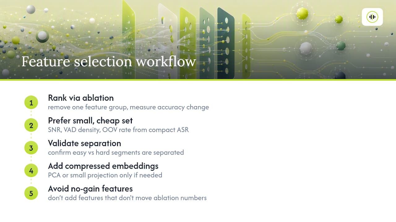
Start by ranking candidate features through ablation, removing one feature group at a time and measuring the resulting change in classifier accuracy. Self-supervised audio embeddings typically carry the most predictive weight, but their high dimensionality (often 512 to 1,024 dimensions per frame) makes them expensive to feed directly into a lightweight classifier. Dimensionality reduction techniques like principal component analysis (PCA) or a small learned projection layer can compress embeddings to a fraction of their original size while retaining most of their discriminative power for routing purposes.
Signal statistics and transcript-derived features are cheap enough that dimensionality reduction matters less for them individually, but combining many low-value features can still add noise to the classifier’s decision boundary. Correlation analysis across your candidate feature set often reveals that SNR, VAD density, and reverberation proxies capture overlapping information, so a well-chosen subset of two or three signal features frequently performs nearly as well as using all of them together.
The practical takeaway for most teams building a first-generation router: start with a small, cheap feature set (SNR, VAD density, OOV rate from a compact ASR pass), validate that it separates easy from hard segments reasonably well, and only add compressed embeddings if the simpler feature set leaves clear routing errors on the table. Adding features that don’t move ablation numbers is pure overhead.
What the Research Actually Supports, and What It Doesn’t
The conventional wisdom in ASR procurement still treats model selection as a one-time decision: benchmark a handful of candidates, pick the leaderboard winner, deploy it everywhere. That approach ignores what the AutoMode-ASR and sample-dependent routing results actually demonstrate, which is that the highest-value gains come from treating selection as a per-segment decision, not a per-project one.
Where the field oversells itself is in assuming a bigger decision module always helps. It doesn’t. The evidence points toward compact, cheap features (signal statistics, a lightweight ASR pass) doing most of the work, with expensive embeddings adding diminishing returns past a certain point. Researchers chasing marginal accuracy gains from heavier feature extractors often lose more to added latency than they gain in routing precision.
If you take one thing from this guide, prioritize the oracle experiment before anything else. It costs almost nothing to run and tells you immediately whether routing is even worth pursuing for your workload, before you invest in a production classifier.
— Benjamin
Prototype Your Routing Strategy in an Afternoon
Building the routing pipeline described above starts with knowing how your candidate models actually perform on your audio, not on someone else’s benchmark. OpenTranscription gives researchers direct access to that comparison: a live model catalog covering 40+ transcription systems with license, language, and streaming metadata, plus a realtime ranking tool that surfaces per-model WER, cost, and speed on the audio you actually care about.
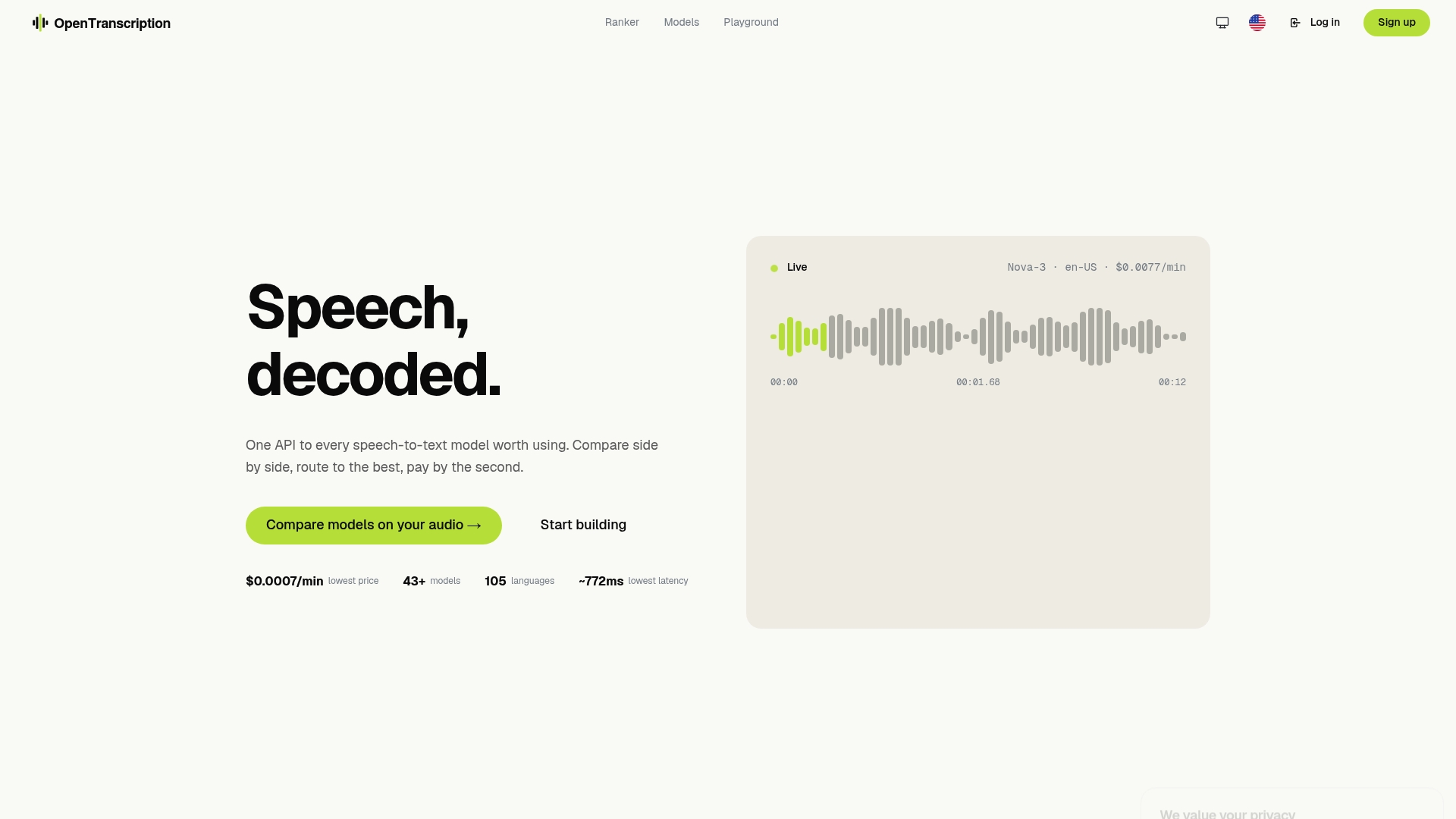
A focused quick-start experiment takes under 90 minutes. Pull a representative 10 to 20 minute sample of your target audio, run it through the model comparison platform to get per-model metrics, then use those results as your first delta-WER labels for a pivot classifier. Because pricing runs per second of audio with no subscription commitment, you can test as many candidate models as your workload needs without negotiating a contract first. Start by comparing your current production model against the catalog to see exactly where a routing layer would pay off.
Sources
- Big model only for hard audios: Sample dependent Whisper model selection for efficient inferences
- Open ASR Leaderboard and standardized benchmarking (arXiv)
- ACL/Computel 2026: Model selection guidance for under-resourced languages
FAQ
What Is an ASR Model?
An ASR (automatic speech recognition) model is a system trained to convert spoken audio into text, typically built on architectures like Conformer, transformer transducers, or CTC decoders that map acoustic input to word or subword sequences.
What Does ASR Stand For?
ASR stands for automatic speech recognition, the general term for technology that transcribes spoken language into written text.
How Does ASR Work?
An ASR system processes audio through an acoustic encoder that extracts speech features, then a decoder that converts those features into text, with modern systems increasingly training both components jointly as end-to-end neural networks.
What Does ASR Stand for in Tech?
In technology contexts, ASR refers specifically to automatic speech recognition systems used in voice assistants, transcription services, call center analytics, and captioning tools rather than any unrelated acronym.
How Do You Choose the Right ASR Model for a Specific Language?
Match candidate models against your target language’s coverage in the model’s training data first, then run a small representative test set through a comparison tool like OpenTranscription’s ranking platform to measure actual WER and cost on your audio rather than relying on published multilingual averages.