
Speaker Diarization: A Developer’s Technical Guide

Speaker diarization answers one precise question: “who spoke when?” The output is a sequence of speaker-labeled timestamps, typically formatted as [SPEAKER_1: 0.0s–4.2s], [SPEAKER_2: 4.2s–7.8s], at either utterance or word level. Every downstream task that depends on attributing speech to individuals, from meeting transcription pipelines to call-center analytics, relies on this labeling step.
Developer use cases where diarization is the critical dependency:
- Meeting transcription pipelines: Segment multi-party recordings into per-speaker turns before passing them to an ASR engine, enabling structured, attributed transcripts.
- Call-center analytics: Separate agent and customer speech for role-aware analysis; role-aware diarization extends blind labeling to assign functional roles like “agent” and “customer.”
- Podcast chaptering and media indexing: Identify speaker transitions to auto-generate chapter markers and searchable speaker segments.
Two reference points worth knowing from the start: DER (Diarization Error Rate) is the standard evaluation metric, and the AMI Meeting Corpus is one of the most widely used benchmark datasets for multi-speaker meeting audio. For teams that want to skip infrastructure setup during early prototyping, OpenTranscription provides an API-driven path to speaker-labeled transcripts across 40+ models.
Table of Contents
- What does a diarization pipeline actually produce?
- How does speaker segmentation differ from diarization?
- What are the core components of a diarization pipeline?
- Cascaded pipelines vs. end-to-end neural diarization: which should you build?
- Which open-source toolkits do developers actually use?
- How do you evaluate diarization, and which datasets should you use?
- Production implementation: the checklist that actually moves the needle
- How does streaming diarization differ from batch processing?
- Common failure modes and how to triage them
- A repeatable methodology for benchmarking diarization approaches
- Key Takeaways
- The part most teams get wrong about diarization rollouts
- OpenTranscription accelerates diarization prototyping and benchmarking
- Useful sources and further reading
What does a diarization pipeline actually produce?
The output of a complete diarization system is a speaker-labeled transcript: each time segment is annotated with a consistent speaker identifier (e.g., SPEAKER_00, SPEAKER_01), either at the utterance level or, when aligned with an ASR system, at the word level. The pipeline that produces this output follows a fixed logical order.
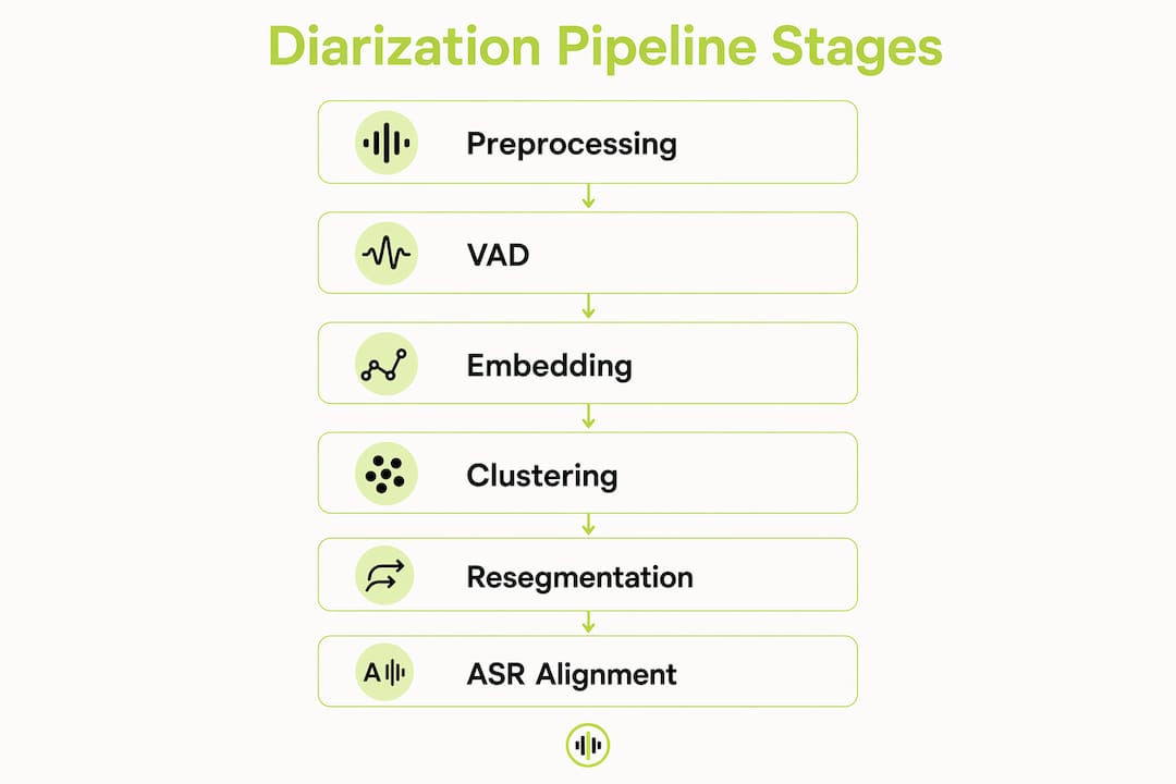
Input → processing → output, step by step:
Raw audio → Voice Activity Detection (VAD) → Segmentation / change-point detection → Embedding extraction → Clustering + resegmentation → Speaker-labeled transcript
Core terms used throughout this guide:
- VAD (Voice Activity Detection): Classifies each audio frame as speech or non-speech; removes silence and noise before further processing.
- Embedding: A fixed-length vector representation of a short audio segment that encodes speaker identity.
- Clustering: Groups embeddings from different segments into speaker clusters, assigning consistent labels.
- Overlap detection: Identifies frames where two or more speakers talk simultaneously.
- Resegmentation: A refinement pass that re-assigns segment boundaries and labels after initial clustering, improving boundary precision.
How does speaker segmentation differ from diarization?
Speaker diarization combines two distinct operations: segmentation and clustering. Treating them as synonymous is one of the most common conceptual errors in pipeline design.
Segmentation detects change points in the audio stream where the speaker identity shifts. Its output is a set of time intervals with no speaker labels attached:
[0.0s–4.2s],[4.2s–7.8s],[7.8s–12.1s]— boundaries only, no identity.
Diarization adds the clustering step, which groups those intervals by speaker identity and assigns consistent labels:
[SPEAKER_1: 0.0s–4.2s],[SPEAKER_2: 4.2s–7.8s],[SPEAKER_1: 7.8s–12.1s]
The practical implication is that errors in a diarization system have two distinct origins, and debugging requires isolating them:
- Bad segmentation produces incorrect boundary placement: a speaker turn is missed entirely, or a boundary is placed mid-utterance. Symptoms include long segments that contain two speakers or very short fragments that split a single utterance.
- Bad clustering produces correct boundaries but wrong identity assignments: two different speakers share a label, or one speaker gets split across multiple labels. Symptoms include DER inflation from speaker confusion rather than missed speech.
When triaging a diarization failure, run segmentation evaluation first. If boundary recall is low, fix VAD and change-point detection before touching the clustering configuration. Clustering errors are only meaningful once segmentation quality is acceptable.
What are the core components of a diarization pipeline?
A production diarization pipeline consists of six ordered stages. Each stage introduces its own failure modes and tuning surface.

1. Audio preprocessing Resample to a consistent rate (typically 16 kHz), convert stereo to mono or process channels independently, and apply loudness normalization. Inconsistent input formats are a frequent source of silent failures.
2. Voice Activity Detection (VAD) VAD classifies each frame as speech or non-speech. Accurate VAD is the single most impactful upstream step: poor VAD generates noisy embeddings from non-speech frames, which corrupt clustering. Common implementations include energy-based detectors, WebRTC VAD, and neural models such as Silero VAD.
3. Segmentation / change-point detection Within speech regions, the system detects speaker transitions. Methods include BIC-based change-point detection, sliding-window cosine distance, and neural segmentation models. The output is a set of homogeneous speech segments.
4. Embedding extraction Each segment is encoded into a speaker embedding vector. Three generations of embeddings are in common use:
- i-vector: Legacy GMM-based approach; low-dimensional, computationally light, but less discriminative under short segments or noise.
- x-vector: TDNN-based, widely used in research and production; strong baseline performance with good community support.
- d-vector / neural embeddings: End-to-end trained speaker representations; more flexible and typically stronger on short segments and accented speech.
5. Clustering Embeddings are grouped into speaker clusters. Agglomerative hierarchical clustering (AHC) with cosine distance is the most common choice. Spectral clustering handles overlapping distributions better in some conditions. K-means variants are used when the speaker count is known in advance.
6. Overlap detection and resegmentation Overlapping speech, where two speakers talk simultaneously, is a major source of DER inflation. A dedicated overlap detection module flags these regions before or after clustering. Resegmentation then refines segment boundaries and re-assigns labels using a Viterbi or HMM-based pass.
7. ASR alignment / label stitching When diarization is combined with automatic transcription, speaker labels are aligned to word-level timestamps from the ASR output, producing a fully attributed transcript.
Pro Tip: Before benchmarking any clustering algorithm, run VAD-only evaluation on your target dataset. Measure the false alarm rate and missed speech rate independently. A VAD false alarm rate above a few percent will inflate DER regardless of how well the downstream clustering performs. Quantify this gap before optimizing anything else.
Cascaded pipelines vs. end-to-end neural diarization: which should you build?
Two dominant system families exist: cascaded (modular) pipelines and end-to-end neural diarization (EEND). The core trade-off is flexibility versus optimization simplicity.
NVIDIA NeMo documentation describes both approaches: cascaded systems offer component-level flexibility and interpretability, while end-to-end models simplify joint optimization and deployment at the cost of some configurability.
| Dimension | Cascaded pipeline | End-to-end neural (EEND) |
|---|---|---|
| Flexibility | High — swap any component independently | Low — monolithic model, harder to modify |
| Debugging | Easier — isolate errors per stage | Harder — errors are entangled across the model |
| Speaker count scaling | Scales to many speakers with AHC | Often constrained to a fixed or small speaker count |
| Overlap handling | Requires explicit overlap module | Can model overlap natively in some architectures |
| Latency | Tunable per component | Depends on model architecture; can be lower |
| Training data requirement | Moderate — components train independently | High — requires large labeled multi-speaker corpora |
| Production maturity | High — well-supported toolkits | Growing — strong research results, fewer production deployments |
Decision checklist:
- Recording length > 30 minutes, speaker count > 6: Cascaded pipeline with AHC scales more reliably.
- Speaker count is small and fixed (2–4), overlap is frequent: EEND architectures handle this better natively.
- Low latency is required: Evaluate both; EEND can be faster when the model is compact, but cascaded streaming pipelines with incremental clustering are well-understood.
- Privacy / on-premise deployment: Both are viable; cascaded pipelines with open-source components (pyannote.audio, NeMo) are easier to deploy on-premise without external dependencies.
- Rapid prototyping: Cascaded pipelines with pre-trained checkpoints (pyannote.audio, NeMo) reach a working baseline faster.
Which open-source toolkits do developers actually use?
Four toolkits dominate practical diarization work in the US research and engineering community. Each has a distinct integration profile.

pyannote.audio
A Python library built on PyTorch, pyannote.audio is the most widely adopted open-source toolkit for diarization research. It provides pre-trained models for VAD, segmentation, overlap detection, and embedding extraction, along with a high-level Pipeline API that runs end-to-end diarization in a few lines of code. Model checkpoints are distributed via Hugging Face Hub. The license requires accepting terms on Hugging Face before downloading pre-trained weights. Quickstart: the pyannote/speaker-diarization-3.1 pipeline on Hugging Face is the canonical starting point.
from pyannote.audio import Pipeline
pipeline = Pipeline.from_pretrained("pyannote/speaker-diarization-3.1",
                                    use_auth_token="YOUR_HF_TOKEN")
diarization = pipeline("audio.wav")
for turn, _, speaker in diarization.itertracks(yield_label=True):
    print(f"{turn.start:.1f}s – {turn.end:.1f}s: {speaker}")
NVIDIA NeMo NeMo provides both cascaded and end-to-end diarization models within a unified framework. Its hands-on notebooks cover ASR-diarization integration, making it the strongest choice when you need attributed transcripts from a single framework. NeMo’s MSDD (Multi-Scale Diarization Decoder) is a well-documented cascaded model with strong benchmark performance. Best fit: teams already using NeMo for ASR who want tight ASR-diarization alignment. Runtime: GPU-accelerated; less practical for CPU-only environments.
Kaldi
Kaldi is a C++ speech toolkit with extensive diarization recipes in the egs/ directory (e.g., egs/callhome_diarization). It is the reference implementation for x-vector extraction and PLDA-based scoring. Integration complexity is high: Kaldi requires familiarity with its shell-script recipe structure and compiled binaries. It is not a Python-native library. Best fit: researchers replicating published baselines or teams that need fine-grained control over every pipeline stage. Community support is active but skews toward academic users.
SpeechBrain SpeechBrain is a PyTorch-based toolkit with VAD tutorials that cover frame-level posterior thresholding, segment merging, and energy-based refinement. Its diarization support is less complete than pyannote.audio out of the box, but its modular design makes it well-suited for building custom pipelines where you want to control VAD and embedding extraction independently. Best fit: teams building custom pipelines who want a clean PyTorch API without the full pyannote.audio abstraction layer.
pyannote community models Beyond the core library, the pyannote community maintains specialized checkpoints for specific conditions (telephone audio, far-field microphones, overlapping speech). These are distributed on Hugging Face and are worth evaluating before training custom models, particularly for domain-specific deployments.
On-premise vs. cloud deployment notes: pyannote.audio and SpeechBrain run entirely on-premise with no external API calls once model weights are downloaded. NeMo is similarly self-contained. Kaldi has no cloud dependency by design. Language support varies: pyannote.audio’s pre-trained models are language-agnostic at the diarization level (they operate on acoustic features, not text), but ASR alignment quality depends on the ASR model’s language coverage.
How do you evaluate diarization, and which datasets should you use?
Core evaluation metrics
DER (Diarization Error Rate) is the primary metric, defined as the fraction of total speech time that is incorrectly labeled. It sums three error components:
- Missed speech: Speech frames labeled as non-speech by VAD.
- False alarm: Non-speech frames labeled as speech.
- Speaker confusion: Speech frames assigned to the wrong speaker.
DER is reported as a percentage; lower is better. Published research often reports DER under “oracle VAD” conditions, where ground-truth speech boundaries are provided, which removes missed speech and false alarm from the score. Production DER with system VAD is consistently higher.
JER (Jaccard Error Rate) measures per-speaker accuracy using the Jaccard similarity between reference and hypothesis speaker regions. JER is less sensitive to dominant speakers than DER and gives a more balanced view of per-speaker performance in multi-speaker recordings.
Speaker-attributed WER applies when diarization is combined with ASR: word error rate is computed per speaker segment, giving a joint measure of transcription and attribution accuracy.
Standard benchmark datasets
| Dataset | Primary use | Audio condition | Notes |
|---|---|---|---|
| AMI Meeting Corpus | Multi-speaker meeting diarization | Far-field, overlapping speech | Standard for meeting transcription benchmarks |
| CALLHOME | Telephony diarization | Telephone channel, 2–7 speakers | Classic benchmark; narrow-band audio |
| VoxCeleb | Speaker embedding training and verification | Diverse, in-the-wild audio | Not a diarization benchmark per se; used for embedding model training |
| LibriCSS | Overlap and continuous speech | Simulated far-field, high overlap | Best for stress-testing overlap detection |
Callout — oracle VAD vs. system VAD: DER numbers reported in papers frequently assume oracle VAD, meaning ground-truth speech boundaries are given to the system. When you replace oracle VAD with a real VAD model, DER typically increases by several percentage points, sometimes substantially. Always measure DER with both oracle and system VAD on your target dataset before drawing conclusions from published benchmarks. The gap between the two numbers tells you exactly how much your VAD is costing you.
Production implementation: the checklist that actually moves the needle
Preprocessing and VAD configuration account for the majority of practical DER improvements in production. Swapping clustering algorithms rarely produces the same gains as fixing upstream issues.
Audio preprocessing checklist:
- Resample all input to 16 kHz; some embedding models (e.g., ECAPA-TDNN in pyannote) are trained at 16 kHz and degrade at other rates.
- Convert stereo to mono by averaging channels unless channel-separated diarization is intended (e.g., telephone with separate agent/customer channels).
- Apply loudness normalization (e.g., EBU R128 or simple peak normalization) to reduce level-dependent VAD errors.
- Trim leading and trailing silence before processing long files.
VAD configuration:
- Set a minimum segment length (typically 0.25–0.5 seconds) to discard spurious short detections; SpeechBrain’s VAD post-processing demonstrates this merge-gap approach explicitly.
- Set a merge-gap parameter (typically 0.1–0.3 seconds) to merge adjacent speech segments separated by short silences, preventing over-fragmentation.
- Tune the posterior threshold on a held-out labeled sample from your target domain; default thresholds from pre-trained models are often calibrated on clean speech and underperform on noisy audio.
Clustering hyperparameter tuning:
- For AHC with cosine distance, sweep the clustering threshold on a development set. A threshold that is too low over-clusters (merges different speakers); too high under-clusters (splits one speaker into multiple labels).
- Use a held-out labeled set of at least 30–60 minutes of audio from your target domain for threshold calibration.
- When the number of speakers is unknown, use automatic speaker count estimation (e.g., eigen-gap analysis for spectral clustering) rather than fixing a count.
Pro Tip: When integrating diarization with ASR for word-level attribution, align speaker segments to word timestamps using a simple interval overlap rule: assign each word to the speaker whose segment covers the largest fraction of that word’s duration. For short turns under 0.5 seconds, consider a look-back window that checks the preceding speaker label to reduce identity flipping on brief back-channel utterances.
How does streaming diarization differ from batch processing?
Batch diarization has access to the full recording before processing begins, which allows global clustering decisions and retrospective boundary refinement. Streaming diarization must assign speaker labels incrementally, with limited or no future context, which introduces a distinct set of failure modes.
The core challenge is identity instability: without future context, the system cannot always determine whether a new voice segment belongs to a previously seen speaker or a new one. This manifests as label flipping, where a speaker’s identity changes mid-session, and as delayed speaker discovery, where a new speaker is not confirmed until enough embedding evidence accumulates.
Streaming architecture options:
- Incremental clustering with a fixed buffer: Maintain a rolling window of recent embeddings and cluster incrementally. Simple to implement; identity instability increases as the session grows and the cluster model drifts.
- Short look-ahead buffer: Delay output by a fixed window (e.g., 1–3 seconds) to allow a small amount of future context before committing to a label. Trades latency for reduced identity flipping.
- Reprocessing windows: Periodically re-run clustering over a recent window (e.g., the last 30–60 seconds) and reconcile labels with the running history. Effective for long sessions; adds CPU cost.
- Hybrid fast-pass + deferred refinement: Emit a preliminary label in real time, then issue a corrected label asynchronously after a short delay. Useful when downstream consumers can handle label corrections.
Latency budget allocation: VAD latency is typically the first bottleneck; a VAD model that processes in 20 ms chunks adds minimal latency. Embedding extraction over a 1.5-second window introduces a minimum latency equal to that window length. Clustering interval (how often you re-run clustering) is the primary tuning knob for the accuracy-latency trade-off. For low-latency applications, the real-time model rankings on OpenTranscription provide a practical reference for comparing streaming transcription and diarization latency across models.
Common failure modes and how to triage them
When DER is higher than expected, the following diagnostic sequence isolates the root cause efficiently.
- Run VAD-only evaluation first. Compute missed speech rate and false alarm rate against ground-truth annotations. If either exceeds your target, fix VAD before proceeding. All downstream metrics are contaminated by VAD errors.
- Visualize segment boundaries. Plot the segmentation output against the reference annotation on a 2–5 minute sample. Identify whether boundaries are missing, misplaced, or over-fragmented.
- Inspect embedding cluster separability. Extract embeddings for all segments and plot them with PCA or t-SNE. If clusters for different speakers overlap significantly, the embedding model is the bottleneck, not the clustering algorithm.
- Test with oracle VAD. Replace your VAD output with ground-truth speech boundaries and re-run diarization. The DER gap between oracle and system VAD quantifies exactly how much VAD is costing you.
- Check overlap detection rates. Compute the fraction of overlapping speech in your dataset. If it exceeds roughly 10–15% of total speech time, and you have no overlap detection module, that alone can explain elevated DER.
- Compute DER with and without overlap allowance. Many evaluation frameworks support a “collar” parameter and an overlap-exclusion flag. Comparing DER with and without overlap regions included isolates the contribution of overlap errors.
- Check for identity hopping. If a single speaker’s label changes multiple times within a session, the embedding window may be too short, or the clustering threshold may be too aggressive. Increase the minimum segment length for embedding extraction and re-evaluate.
Common root causes and fixes:
- Identity hopping: Increase embedding window length; improve VAD to reduce fragmented segments; raise the clustering merge threshold.
- Over-clustering (one speaker split into multiple labels): Lower the AHC distance threshold; increase the minimum cluster size.
- Under-clustering (multiple speakers merged): Raise the AHC distance threshold; verify embedding model is appropriate for your audio domain.
- High missed speech: Retune VAD posterior threshold downward on your target domain; check for domain mismatch between VAD training data and your audio.
- High false alarm: Raise VAD threshold; apply minimum segment length post-processing.
A repeatable methodology for benchmarking diarization approaches
Reproducible benchmarking requires explicit control over every variable that affects DER. The following protocol covers the decisions that most often cause irreproducible results.
Dataset and data preparation:
- Select a dataset appropriate for your target condition (AMI for meetings, CALLHOME for telephony, LibriCSS for overlap-heavy audio).
- Define a fixed train/dev/test split and never tune hyperparameters on the test set.
- Document the exact audio format: sample rate, channel count, encoding, and any preprocessing applied.
VAD policy:
- Run all comparisons under both oracle VAD and system VAD conditions and report both.
- Use the same VAD model and configuration across all compared systems; changing VAD between systems conflates VAD quality with diarization quality.
Metric selection and reporting:
- Report DER as the primary metric; include JER when per-speaker balance matters.
- Specify the collar value (typically 0.25 seconds) and whether overlapping speech regions are included or excluded.
- Report results on the full test set, not cherry-picked subsets.
Experiment configuration to record:
- Sampling rate and channel handling
- Frame shift and window size for embedding extraction
- Embedding model name and version (e.g.,
pyannote/embeddingcheckpoint hash) - Clustering algorithm, distance metric, and threshold value
- Overlap detection: enabled/disabled, model version
- Minimum segment length and merge-gap values
- Random seed for any stochastic components
Reproducibility:
- Fix random seeds for all stochastic steps (clustering initialization, data shuffling).
- Log compute budget: GPU/CPU type, wall-clock time per experiment.
- Publish a configuration file (YAML or JSON) alongside results so others can replicate the exact run.
- For significance testing, run multiple seeds and report mean and standard deviation of DER across seeds.
Key Takeaways
Speaker diarization requires accurate VAD as its foundation: fixing upstream speech detection consistently produces larger DER improvements than tuning clustering algorithms.
| Point | Details |
|---|---|
| VAD quality drives DER | Measure missed speech and false alarm rates before optimizing any other pipeline component. |
| Oracle vs. system VAD gap | Always report DER under both conditions; the gap quantifies your VAD’s production cost. |
| System type by use case | Use cascaded pipelines for large speaker counts and flexibility; consider EEND for small, fixed speaker counts with frequent overlap. |
| Standard datasets and metrics | Benchmark on AMI, CALLHOME, or LibriCSS with DER and JER; match the dataset to your target audio condition. |
| OpenTranscription for prototyping | OpenTranscription’s API provides speaker-labeled transcripts across 40+ models with per-second billing, accelerating benchmarking without infrastructure setup. |
The part most teams get wrong about diarization rollouts
Most teams approach a diarization project as a model selection problem. They spend the first two weeks evaluating pyannote.audio against NeMo, reading benchmark tables, and debating x-vectors versus d-vectors. Then they integrate the chosen toolkit, run it on their actual audio, and discover that DER is 15 percentage points higher than the published benchmark. The culprit is almost never the clustering algorithm.
In practice, the first month of a diarization project should be almost entirely about data and preprocessing. Collect 30–60 minutes of labeled audio from your exact target domain, run VAD-only evaluation, and measure the gap between oracle and system VAD. That number tells you more about your project’s difficulty than any benchmark table. Teams that skip this step consistently underestimate the effort required to reach production-grade accuracy.
The second phase, once VAD is acceptable, is overlap detection. Overlapping speech is underrepresented in most benchmark datasets relative to real-world conditions, particularly in meeting and call-center audio. Adding an explicit overlap detection module, even a simple one, often reduces DER more than any clustering improvement at this stage.
The third phase is ASR integration. Aligning speaker labels to word-level timestamps introduces its own failure modes: short back-channel utterances, cross-talk, and speaker label instability across long sessions. Instrument DER per release from the start, and set alerting thresholds on speaker stability metrics before you reach production scale. A DER that drifts upward across software releases is a signal that a preprocessing or model version change has introduced a regression, and catching it early is far cheaper than diagnosing it after deployment.
OpenTranscription accelerates diarization prototyping and benchmarking
Building and maintaining a full open-source diarization stack takes time: model weight management, VAD tuning, embedding pipeline configuration, and ASR alignment all require sustained engineering effort before you see a labeled transcript. For teams at the prototyping or benchmarking stage, that infrastructure cost delays the actual research question.
OpenTranscription provides a direct alternative: an API that delivers speaker-labeled, structured transcripts with word-level timestamps across 40+ transcription models, billed per second of audio with no subscription required. You can run the same audio file through multiple diarization-capable models in a single session, compare DER-relevant outputs side by side, and identify which model fits your audio condition before committing to an infrastructure build. Real-time streaming support means you can evaluate latency-accuracy trade-offs on live audio without building a streaming pipeline first. For teams with privacy or on-premise requirements, the platform supports bring-your-own-provider billing and enterprise deployment options.
The practical use case: take a representative 30-minute sample from your target domain, run it through the model catalog on OpenTranscription, and use the structured output to calibrate your evaluation before investing in a full open-source stack.
Useful sources and further reading
- NIST RT Evaluation: The original source for DER definition and evaluation protocols; essential reading for understanding how benchmark numbers are computed and what assumptions they carry.
- AMI Meeting Corpus: Dataset documentation and download instructions for the standard meeting diarization benchmark; includes both close-talk and far-field microphone recordings.
- CALLHOME LDC catalog: Telephony diarization dataset; the reference for narrow-band, two-to-seven-speaker benchmarks.
- LibriCSS LDC catalog: Overlap-focused continuous speech dataset; use this when stress-testing overlap detection modules.
- pyannote.audio GitHub: Primary repository for the pyannote toolkit; contains model cards, pipeline configurations, and community checkpoint links on Hugging Face.
- NVIDIA NeMo diarization docs: Official documentation covering both cascaded and end-to-end diarization models, with Jupyter notebook tutorials for ASR-diarization integration.
- SpeechBrain VAD tutorial: Step-by-step tutorial covering frame-level VAD, posterior thresholding, and segment post-processing; directly applicable to the VAD configuration checklist above.
- Aalto VAD chapter: Academic treatment of VAD theory and its role in speech processing pipelines; useful background for understanding why VAD quality propagates through the entire diarization system.
- OpenTranscription blog: Applied model-by-model analysis and benchmarks, including coverage of real-time speech-to-text models relevant to streaming diarization evaluation.