Real-Time Diarization for Developers: Practical Guide

Real-Time Diarization for Developers: Practical Guide

For most production use cases, the recommended real-time diarization approach is incremental clustering with a rolling buffer (500ms–2s) combined with ASR word-level alignment. The core trade-off is direct: streaming diarization yields a clearly higher DER than offline batch processing because the model lacks global context across the full audio. That penalty is acceptable when the user experience demands immediate speaker attribution; it is not acceptable when accuracy is the primary constraint and latency is secondary.

When to choose streaming vs. batch:

• Streaming real-time diarization: live transcription interfaces, call center agent assist, meeting captioning, voice-controlled applications where speaker labels must appear within one to two seconds of speech.
• Batch offline diarization: post-call analytics, legal transcription, research corpora where DER must be minimized and processing time is unconstrained.

Minimal POC stack to start today:

• WebSocket client sending 100ms audio frames at real-time pace
• Server-side rolling buffer of 500ms–2s for low-latency, or up to 5s for better DER
• Speaker embeddings (x-vector or ECAPA-TDNN family) with incremental clustering
• Cannot-link constraints to prevent short-term cluster merges
• ASR alignment layer to attach speaker labels to word-level timestamps

Pro Tip: Before committing to a streaming architecture, run your target audio through an offline pipeline first. The offline DER is your accuracy ceiling; the streaming DER will be 10–15% higher. If the offline result is already poor on your audio domain, fix the model before adding streaming constraints.

---

Table of Contents

• How do you build a minimal real-time diarization pipeline?
• What architecture pattern should you choose for streaming diarization?
• Which models and libraries support real-time speaker diarization?
• How do you align diarized speaker segments with ASR word-level timestamps?
• How do you measure streaming diarization quality accurately?
• How do you reduce streaming diarization latency without wrecking accuracy?
• What goes wrong in streaming diarization deployments, and how do you fix it?
• OpenTranscription’s benchmark summary and recommended production pipeline
• Key Takeaways
• When should you build in-house versus use a managed streaming API?
• OpenTranscription makes streaming diarization production-ready
• Useful sources and documentation to read next

How do you build a minimal real-time diarization pipeline?

A working end-to-end pipeline has five stages: audio capture, chunked streaming, incremental diarization, ASR transcription, and speaker-labeled output. The prerequisites are modest for a proof-of-concept: Python 3.10+, a CUDA-capable GPU (optional but recommended for sub-200ms embedding inference), and a test audio file with at least two speakers and some natural overlap.

Required libraries for a local POC:

• pyannote.audio for speaker embeddings and segmentation
• websockets or aiohttp for the streaming transport layer
• diart for the rolling-buffer incremental clustering loop
• A speech recognition SDK (e.g., azure-cognitiveservices-speech or the Deepgram Python SDK) for ASR alignment
• numpy and torch for embedding computation

Recommended test audio: AMI meeting corpus recordings or LibriSpeech multi-speaker mixes give reproducible baselines. Avoid synthetic TTS audio for diarization tests; the embedding distributions differ from natural speech.

WebSocket client: 100ms frame streaming

The client reads audio in 100ms chunks and sends each frame at real-time pace. Sending faster than the real-time clock is the single most common cause of server-side connection drops, because servers typically enforce a 5-second buffer limit and will close the connection if the client races ahead.

import asyncio
import websockets
import soundfile as sf
import numpy as np

CHUNK_DURATION_S = 0.1   # 100ms
SAMPLE_RATE = 16000
CHUNK_SAMPLES = int(SAMPLE_RATE * CHUNK_DURATION_S)

async def stream_audio(uri: str, audio_path: str):
    audio, sr = sf.read(audio_path, dtype="float32")
    assert sr == SAMPLE_RATE, f"Resample to {SAMPLE_RATE} Hz first"

    async with websockets.connect(uri) as ws:
        for start in range(0, len(audio), CHUNK_SAMPLES):
            chunk = audio[start : start + CHUNK_SAMPLES]
            await ws.send(chunk.tobytes())
            await asyncio.sleep(CHUNK_DURATION_S)   # pace to real time

        await ws.send(b"end_of_stream")             # flush final segments
        response = await ws.recv()
        print("Final transcript:", response)

asyncio.run(stream_audio("ws://localhost:8765", "meeting.wav"))

Minimal server sketch with incremental clustering

On the server side, a diart-based pipeline receives each chunk, updates the rolling buffer, runs speaker segmentation and embedding, and emits incremental speaker labels. The diart framework implements cannot-link constraints natively, preventing the clustering algorithm from merging two speakers who were active in the same short window.

from diart import SpeakerDiarization
from diart.sources import AudioSource
import asyncio, websockets

pipeline = SpeakerDiarization()  # uses default rolling buffer ~500ms

async def handle_client(ws, path):
    source = AudioSource(sample_rate=16000)
    async for message in ws:
        if message == b"end_of_stream":
            source.close()
            break
        source.push(message)
    for annotation, audio in pipeline(source):
        await ws.send(str(annotation))

asyncio.run(websockets.serve(handle_client, "localhost", 8765))

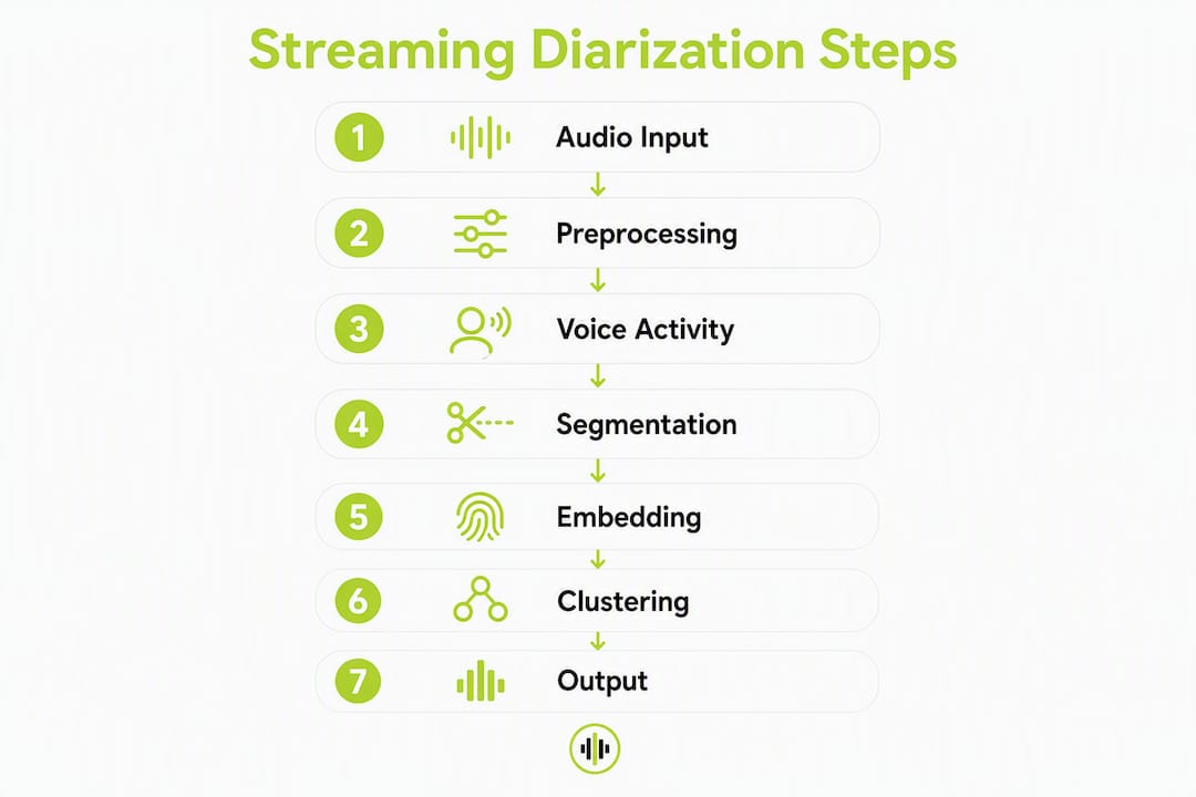
Dataflow sequence:

1. Microphone or file reader produces raw PCM at 16 kHz.
2. Client segments into 100ms frames and sends over WebSocket at real-time pace.
3. Server accumulates frames into a rolling buffer (500ms–2s).
4. Segmentation model (e.g., pyannote segmentation-3.0) identifies speech regions.
5. Embedding model (ECAPA-TDNN or similar) encodes each segment.
6. Incremental clustering assigns or creates speaker IDs with cannot-link constraints.
7. ASR layer aligns speaker IDs with word-level timestamps.
8. Labeled transcript emitted to client.

Key implementation detail: Always send an explicit end_of_stream signal rather than abruptly closing the WebSocket. An abrupt close causes the server to discard buffered audio that has not yet been processed, which typically drops the last 500ms–2s of speech and corrupts the final speaker segment attribution.

Pro Tip: For short-term clustering stability during the first 3–5 seconds of a stream, seed the cannot-link constraint matrix with any known speaker embeddings from a prior session or enrollment step. Cold-start confusion is highest in the first buffer window.

---

What architecture pattern should you choose for streaming diarization?

Three paradigms cover the design space: modular pipeline, end-to-end neural diarization (EEND), and hybrid approaches. Each has a distinct latency profile, accuracy ceiling, and engineering complexity.

Modular pipeline (VAD → segmentation → embeddings → clustering)

The modular approach chains discrete components. Voice activity detection (VAD) identifies speech regions; a segmentation model finds speaker change points; an embedding model encodes each segment; a clustering algorithm groups embeddings into speaker identities. Each component can be swapped independently, which makes debugging and incremental improvement tractable. The main streaming liability is accumulated latency across the chain: each stage adds processing time, and the clustering step requires a minimum buffer of speech before it can make stable assignments.

End-to-end neural diarization (EEND)

EEND models, such as the EEND-EDA family, process raw features and emit speaker activity probabilities directly without explicit clustering. They handle overlapping speech natively because they model multiple simultaneous speakers as a multi-label output. The trade-off for streaming is that EEND models were originally designed for fixed-length inputs; online variants (EEND-online) use chunked inference with a recurrent state, which introduces permutation ambiguity across chunks. Architectures like Sortformer v2 address this with streaming caches that maintain speaker identity across chunk boundaries, achieving real-time factors exceeding 200x in benchmarking.

Hybrid approaches

Hybrid systems combine EEND-style overlap detection with modular clustering for speaker tracking. A common pattern: EEND handles the overlap detection and short-segment classification; a separate embedding-clustering module maintains global speaker identity across the full stream. This delivers better overlap handling than pure modular systems without the permutation instability of pure EEND in long streams.

Architecture	Overlap handling	Streaming latency	Speaker count scalability	Compute requirement	Best fit
Modular pipeline	Poor to moderate	Medium (200ms–1s)	High (no fixed limit)	CPU feasible	Multi-speaker meetings, call diarization
EEND (online)	Excellent	Low (100–300ms)	Limited (typically ≤4)	GPU required	Two-speaker calls, interview audio
Hybrid	Good	Medium (300ms–5000ms)	Moderate (≤8)	GPU recommended	Meeting transcription with overlap

Decision checklist before choosing an architecture:

• Target latency under 300ms: lean toward EEND-online or a lightweight modular pipeline with a 500ms buffer.
• More than four concurrent speakers expected: modular or hybrid; EEND degrades with speaker count.
• Significant overlap expected (>15% of audio): EEND or hybrid for better multi-label detection.
• CPU-only deployment: modular pipeline with lightweight segmentation (e.g., silero-VAD + small embedding model).
• Online speaker enrollment needed: modular pipeline; EEND cannot incorporate new speaker embeddings at inference time.

Pro Tip: Profile your target audio domain before selecting an architecture. Meeting audio with frequent overlaps favors hybrid; two-party phone calls favor EEND-online; large conference calls with up to 12 speakers favor modular with a high-capacity clustering backend.

---

Which models and libraries support real-time speaker diarization?

The open-source and managed-service options differ substantially in integration complexity, resource footprint, and the latency floor they can realistically achieve.

Open-source toolkits:

• pyannote.audio: The most widely adopted open-source diarization library. Publishes pretrained pipelines on Hugging Face and supports GPU-accelerated inference. The pyannote/speaker-diarization-3.1 pipeline is the current-recommended starting point for offline use; for streaming, diart wraps pyannote models in a rolling-buffer loop. GPU is strongly recommended for real-time embedding inference; CPU-only setups typically exceed 1s latency per chunk.
• diart: A streaming-first wrapper around pyannote models that implements the rolling-buffer pattern and cannot-link constraints out of the box. Latency is configurable from 500ms to 5s. The lower bound is suitable for live captioning; the upper bound trades latency for DER reduction.
• NeMo (NVIDIA): NVIDIA’s NeMo toolkit includes the Sortformer family of diarization models. Sortformer v2 is designed with streaming caches and achieves real-time factors well above 1x, making it viable for low-latency deployment on NVIDIA hardware. Integration complexity is higher than pyannote for non-NVIDIA environments.
• silero-VAD: A lightweight VAD model that runs efficiently on CPU and is commonly used as the first stage in a modular pipeline to reduce the embedding workload by filtering non-speech frames. Not a full diarization system, but a critical preprocessing component.

Managed streaming APIs:

• Microsoft Azure Speech Service: Publishes a real-time diarization quickstart using the Conversation Transcriber, which exposes a SpeakerId field on each recognition result. The managed service handles chunking, embedding, and clustering server-side; the client SDK (azure-cognitiveservices-speech) abstracts the WebSocket transport. Suitable for enterprise deployments where operational overhead must be minimized.
• AssemblyAI: Offers real-time transcription with speaker labels via a WebSocket API. The speaker diarization is applied post-recognition on the server side, so the latency for speaker attribution is slightly higher than for the transcript itself. Well-documented for Python and Node.js integrations.
• Deepgram: Provides streaming transcription with diarization enabled via a query parameter. The Deepgram Flux model integrates turn detection at the model level, reducing the need for a separate segmentation stage. Deepgram’s Nova and Base model families offer different latency/accuracy trade-offs; the Deepgram Base profile documents the lower-resource option.
• OpenTranscription: Provides a unified streaming API that routes requests across 40+ transcription models, including those with real-time diarization support. The realtime model rankings page benchmarks models by latency, accuracy, and cost, allowing engineers to select the right model for a specific SLA without running their own benchmark suite.

Tool	Real-time support	GPU required	Integration complexity	Language support
pyannote.audio + diart	Yes (rolling buffer)	Recommended	Medium	Multilingual
NeMo Sortformer v2	Yes (streaming cache)	Yes (NVIDIA)	High	English-primary
Azure Speech Service	Yes (managed)	No (cloud)	Low	100+ languages
AssemblyAI	Yes (managed)	No (cloud)	Low	Multiple
Deepgram	Yes (managed)	No (cloud)	Low	30+ languages
OpenTranscription API	Yes (managed, multi-model)	No (cloud)	Low	105+ languages

Pro Tip: Preprocessing effects are model-dependent — background separation that improves DER on one model can degrade it on another. Always validate any preprocessing step on a held-out sample of your target audio before applying it in production.

---

How do you align diarized speaker segments with ASR word-level timestamps?

Producing a speaker-labeled transcript requires merging two output streams: diarization segments (speaker ID, start time, end time) and ASR word-level timestamps (word, start time, end time, confidence). The alignment is not trivial in a streaming system because the two streams may have different latencies and different temporal resolutions.

Two integration patterns:

Pattern 1: Post-hoc alignment. The ASR engine and diarization pipeline run independently. After both produce output for a buffer window, a reconciliation step maps each ASR word to the speaker whose diarization segment has the maximum overlap with that word’s time span. This is the simpler pattern and works well when both streams have similar latency. The risk is drift: if diarization lags ASR by more than 200ms, words near speaker boundaries get misattributed.

Pattern 2: Tightly coupled pipeline. The ASR model emits word-level timestamps in real time, and the diarization engine is queried synchronously for the speaker ID at each word’s midpoint timestamp. This requires both systems to share a common clock and buffer state. Azure’s Conversation Transcriber uses this pattern, attaching SpeakerId directly to each recognition result as it arrives.

Handling speaker label drift:

• Buffer ASR words for 300–500ms after they are emitted before finalizing speaker attribution, giving the diarization engine time to stabilize its cluster assignment for that time window.
• Use exclusive speaker labels: each word gets exactly one speaker ID, even in overlap regions. Assign the word to the speaker with the highest diarization confidence score for that timestamp.
• Track speaker ID mapping across buffer windows. Incremental clustering can reassign cluster indices between windows; maintain a stable mapping from cluster index to canonical speaker label (e.g., SPEAKER_00, SPEAKER_01) using a Hungarian algorithm or a simple nearest-neighbor match on embeddings.

Step-by-step alignment procedure:

1. Collect ASR word objects: {word, start_ms, end_ms, confidence}.
2. Collect diarization segments: {speaker_id, start_ms, end_ms} from the current buffer window.
3. For each word, compute overlap with all active diarization segments.
4. Assign the word to the speaker with maximum overlap; if no segment covers the word’s midpoint, assign to the nearest segment by start time.
5. Emit the labeled word: {word, speaker_id, start_ms, end_ms, confidence}.
6. After the buffer window closes, finalize and flush labeled words to the output stream.

Alignment step	Key parameter	Failure mode	Mitigation
Word buffering delay	300–500ms	Words emitted before speaker stabilizes	Increase buffer; accept higher output latency
Overlap resolution	Exclusive label per word	Overlap words misattributed	Use confidence-weighted assignment
Speaker ID mapping	Cluster-to-label map	Label flip across windows	Embedding nearest-neighbor re-identification
Drift correction	Clock sync tolerance	Systematic offset between ASR and diarization	Shared timestamp source; NTP sync on server

---

How do you measure streaming diarization quality accurately?

Diarization Error Rate (DER) is the standard metric. It decomposes into three additive components: missed speech (speech the model labels as silence), false alarm (silence labeled as speech), and speaker confusion (speech attributed to the wrong speaker). In streaming systems, missed speech is typically the dominant failure mode, with average missed durations around 350ms per segment observed across multiple model families in published benchmarks.

Jaccard Error Rate (JER) is a complementary metric that weights each speaker equally regardless of speaking time, making it more sensitive to errors on minority speakers. DER can look acceptable on a recording dominated by one speaker even when secondary speakers are poorly tracked; JER surfaces those failures.

Collar trimming (typically 0.25s) removes a window around each speaker boundary from the evaluation, acknowledging that boundary placement is inherently ambiguous. Always report whether a collar was applied and its value; results without a collar are not directly comparable to results with one.

Recommended datasets for streaming benchmark design:

• AMI Meeting Corpus: Multi-speaker meeting audio with reference annotations; widely used for DER benchmarking.
• CALLHOME: Two-speaker telephone conversations; useful for call diarization evaluation.
• VoxConverse: In-the-wild audio from YouTube; tests robustness to noise and channel variation.
• Synthetic multi-speaker mixes: Useful for controlled overlap-rate experiments, but not a substitute for real-world audio.

Benchmark design checklist for reproducible streaming tests:

• Fix the random seed for any stochastic components (clustering initialization, data augmentation).
• Use a fixed chunk size (100ms) and fixed buffer size across all runs.
• Measure and report end-to-end latency from audio frame arrival to speaker label emission, not just model inference time.
• Report DER with and without the skip_overlap option so readers can assess overlap handling separately.
• Record GPU/CPU utilization and memory peak alongside accuracy metrics.

Metric	Definition	Typical streaming range	Notes
DER (no collar)	(missed + false alarm + confusion) / total speech	15%	Higher in streaming vs. offline
DER (0.25s collar)	DER excluding boundary regions	10–25%	Standard for published comparisons
JER	Per-speaker Jaccard error, averaged	20–40%	More sensitive to minority speakers
Latency	Label emission delay	200ms–2s	Depends on buffer size
RTF	Processing time / audio duration	<1.0 for real-time	Sortformer v2 exceeds 200x RTF

Benchmark design note: Streaming DER is not directly comparable to offline DER from the same model. Always run both evaluations on the same audio to quantify the streaming penalty for your specific system before reporting results.

---

How do you reduce streaming diarization latency without wrecking accuracy?

The rolling buffer size is the primary engineering lever. A 500ms buffer minimizes latency but gives the clustering algorithm very little context, which increases speaker confusion and permutation errors. A 5s buffer reduces DER substantially but introduces a 5s speaker attribution lag, which is unacceptable for live captioning. Most production systems settle between 1s and 2s as a practical compromise.

Concrete optimization tactics:

• Lightweight segmentation model: Replace a heavy transformer segmentation model with silero-VAD for the first-pass speech/non-speech decision. silero-VAD runs on CPU in under 10ms per 100ms chunk, freeing GPU cycles for the embedding model.
• Lower-dimension embeddings: Reduce ECAPA-TDNN output from 192 to 64 dimensions. The DER increase is typically small on clean audio; the embedding computation and clustering time drop proportionally.
• GPU vs. CPU trade-offs: Embedding inference on a mid-range GPU (e.g., NVIDIA T4) runs 10–20x faster than on a modern CPU for batch sizes above 4. For single-stream deployments, a CPU with AVX-512 support can sustain real-time embedding at 16 kHz with a 500ms buffer if the model is quantized.
• INT8 quantization: Quantizing the embedding model to INT8 reduces memory bandwidth and compute by roughly half with minimal accuracy loss on speaker verification tasks. Apply quantization after validating DER on your target audio domain, not before.
• Frame skipping: Process every other 10ms frame in the segmentation model during low-energy regions (below a VAD confidence threshold). This reduces compute by up to 40% on audio with significant silence, at negligible DER cost.
• Adaptive buffering: Monitor the real-time factor (RTF) of the pipeline. If RTF approaches 1.0, increase the buffer window to batch more frames per inference call, reducing per-frame overhead at the cost of slightly higher latency.

Latency target	Buffer size	Expected DER increase vs. offline	Recommended hardware
<300ms	500ms	+15–20%	GPU (T4 or better)
300ms–1s	1s	+12–15%	GPU or high-end CPU
1s–3s	2s	+10–12%	CPU feasible with quantization
3s–5s	5s	+8–10%	CPU

Pro Tip: Instrument your pipeline with per-stage latency histograms (VAD, embedding, clustering, ASR alignment) from day one. The bottleneck is rarely where engineers expect it; embedding inference and clustering are usually the dominant contributors, not the WebSocket transport.

---

What goes wrong in streaming diarization deployments, and how do you fix it?

Most streaming diarization failures fall into five categories: connection drops, buffer overflows, speaker label drift, missed speech segments, and overlap misattribution. Each has a distinct root cause and a targeted fix.

Troubleshooting checklist:

• Connection drops: Almost always caused by sending audio faster than real time. Add a sleep(chunk_duration) after each send call. Verify with server logs that the client is not racing ahead of the real-time clock.
• Buffer overflows: The server’s 5s buffer fills when the client sends a burst (e.g., after a network pause). Implement client-side pacing with a token bucket or leaky bucket rate limiter. If the server closes the connection, reconnect and resume from the last acknowledged timestamp.
• Speaker label drift: Cluster indices reassigned between buffer windows cause the same physical speaker to appear under two different labels. Maintain a persistent embedding centroid per speaker label and re-identify clusters at each window boundary using cosine similarity.
• Missed speech segments: Short utterances (under 500ms) are frequently missed because they fall below the segmentation model’s minimum segment duration. Reduce the minimum segment duration parameter in the segmentation model, or use a more sensitive VAD as a pre-filter.
• Overlap misattribution: Words spoken simultaneously by two speakers get assigned to one speaker. Enable overlap detection in the segmentation model if supported, or apply a hybrid architecture that handles multi-label output.

Step-by-step debugging procedure for a new deployment:

1. Stream a known reference file (e.g., an AMI segment with published DER) and compare your system’s output DER to the published value.
2. Isolate each pipeline stage by logging timestamps at VAD output, embedding output, clustering output, and ASR alignment output.
3. Reproduce failures with synthetic test cases: a 200ms utterance (tests short-segment handling), a 2s overlap region (tests overlap detection), and a 30s silence gap (tests reconnection and buffer reset).
4. Apply cannot-link constraints if speaker confusion is the dominant DER component.
5. If missed speech is dominant, increase VAD sensitivity or reduce the minimum segment duration threshold.

Operational note: Log every end_of_stream signal and the corresponding final segment count. A mismatch between expected and received final segments is the fastest diagnostic for buffer-flush failures, which are otherwise silent and difficult to detect from transcript output alone.

Remediation patterns for common failure modes:

• Cannot-link constraints (diart): prevent merging of speakers active in the same 500ms window; reduces confusion DER by 2–5 percentage points in typical meeting audio.
• Increased buffer window: moving from 500ms to 2s typically reduces speaker confusion at the cost of higher output latency.
• Enhanced VAD pre-filtering: silero-VAD before the segmentation model reduces false alarm rate and lightens the embedding workload.
• Noise separation as preprocessing: test preprocessing effects per model before deploying; background separation degrades some models trained on noisy data.

---

OpenTranscription’s benchmark summary and recommended production pipeline

A reproducible benchmark for streaming diarization compares systems on the same audio under identical chunking and buffer conditions. Public benchmarks on the AMI and VoxConverse corpora show that modular pipelines with 2s rolling buffers achieve DER in the 15–25% range on meeting audio without collar trimming, while managed APIs with server-side optimization typically land in a similar range with lower operational overhead. The Sortformer v2 architecture demonstrates that streaming-cache designs can achieve real-time factors exceeding 200x, establishing a practical upper bound on throughput for GPU-accelerated deployments.

Recommended production pipeline:

• Stage 1: silero-VAD for speech/non-speech filtering (CPU, <10ms per 100ms chunk).
• Stage 2: pyannote segmentation-3.0 or equivalent for speaker change detection (GPU recommended).
• Stage 3: ECAPA-TDNN embeddings with cannot-link constraints via diart (GPU recommended, 500ms–2s buffer).
• Stage 4: ASR alignment using a streaming-capable model with word-level timestamps.
• Stage 5: Monitoring hooks: per-stage latency histograms, RTF tracking, and DER spot-checks on sampled audio.

OpenTranscription integrates with this flow at Stage 4 and, optionally, as a full replacement for Stages 2–4 via its streaming API. The model catalog lists all supported models with their latency, accuracy, and cost profiles, allowing engineers to select the right model for a specific SLA without running a full benchmark suite internally. For teams needing to compare multiple ASR backends under identical streaming conditions, the realtime rankings page provides side-by-side latency and accuracy data.

When to use the OpenTranscription streaming API vs. self-hosting:

• Use OpenTranscription for production: when operational overhead, model maintenance, and multi-language support (105+ languages) are constraints; when per-second billing is preferable to GPU infrastructure costs; when you need reproducible model profiles without running your own benchmark suite.
• Self-host for research: when you need full control over model weights, training data, and evaluation conditions; when your audio domain is highly specialized and requires fine-tuning; when data privacy constraints prohibit sending audio to a third-party API.

Pro Tip: Run a 30-minute AMI segment through both your self-hosted pipeline and the OpenTranscription streaming API before committing to either path. The DER difference on your specific audio domain is more informative than any published benchmark, because domain mismatch is the largest single source of production DER degradation.

---

Key Takeaways

Streaming diarization incurs a 10–15% DER penalty versus offline processing; the rolling buffer size, cannot-link constraints, and ASR alignment strategy are the three levers that most directly control where your system lands within that penalty range.

Point	Details
Streaming DER penalty	Expect 10–15% higher DER than offline; only use streaming when low-latency speaker attribution is required by the UX.
Rolling buffer trade-off	A 500ms buffer minimizes latency but increases speaker confusion; a 2s buffer is the practical production default for most meeting and call use cases.
Cannot-link constraints	Applying cannot-link constraints in incremental clustering reduces speaker confusion DER by 2–5 percentage points without increasing latency.
ASR alignment strategy	Buffer ASR words for 300–500ms before finalizing speaker attribution to allow diarization cluster assignments to stabilize at speaker boundaries.
OpenTranscription API	The realtime model rankings and model catalog let engineers select and benchmark streaming models by latency, accuracy, and cost without building an internal benchmark suite.

---

When should you build in-house versus use a managed streaming API?

The build-vs-buy decision for real-time diarization is less about capability and more about operational cost and time-to-market. Self-hosting a pyannote or NeMo pipeline gives full control over model weights, training data, and evaluation conditions, which matters for specialized audio domains (clinical interviews, courtroom recordings, low-resource languages) where pretrained models underperform and fine-tuning is necessary. The operational burden is real: GPU infrastructure, model versioning, monitoring, and the latency of keeping up with upstream model releases all accumulate into engineering hours that compound over time.

Managed APIs eliminate that operational layer entirely, but they introduce a different constraint: you are dependent on the provider’s model update cadence and pricing model. For most product teams shipping a live transcription feature, the managed path is the correct default. The DER difference between a well-configured managed API and a self-hosted pipeline on general-domain audio is typically within the measurement noise of a realistic production benchmark, and the time saved on infrastructure is better spent on product-layer features.

The case for building in-house is strongest when the audio domain is narrow and specialized, when data privacy regulations prohibit third-party processing, or when the team has a specific research objective that requires access to intermediate model outputs (embeddings, segmentation posteriors) that managed APIs do not expose. Even then, the practical recommendation is to start with a managed API to establish a DER baseline, then build in-house only when that baseline is demonstrably insufficient for the target use case.

Reproducible benchmarking before any rollout decision is non-negotiable. A DER measured on AMI or VoxConverse tells you almost nothing about performance on your specific audio. Run your own evaluation on a representative held-out sample, measure latency under realistic network conditions, and document the results before committing to either path.

---

OpenTranscription makes streaming diarization production-ready

Deploying a real-time diarization pipeline from scratch means managing GPU infrastructure, model versioning, WebSocket transport, and benchmark tooling simultaneously. OpenTranscription removes that overhead by providing a unified streaming API that routes across 40+ transcription models, including those with real-time speaker diarization support, billed per second of audio with no subscription lock-in.

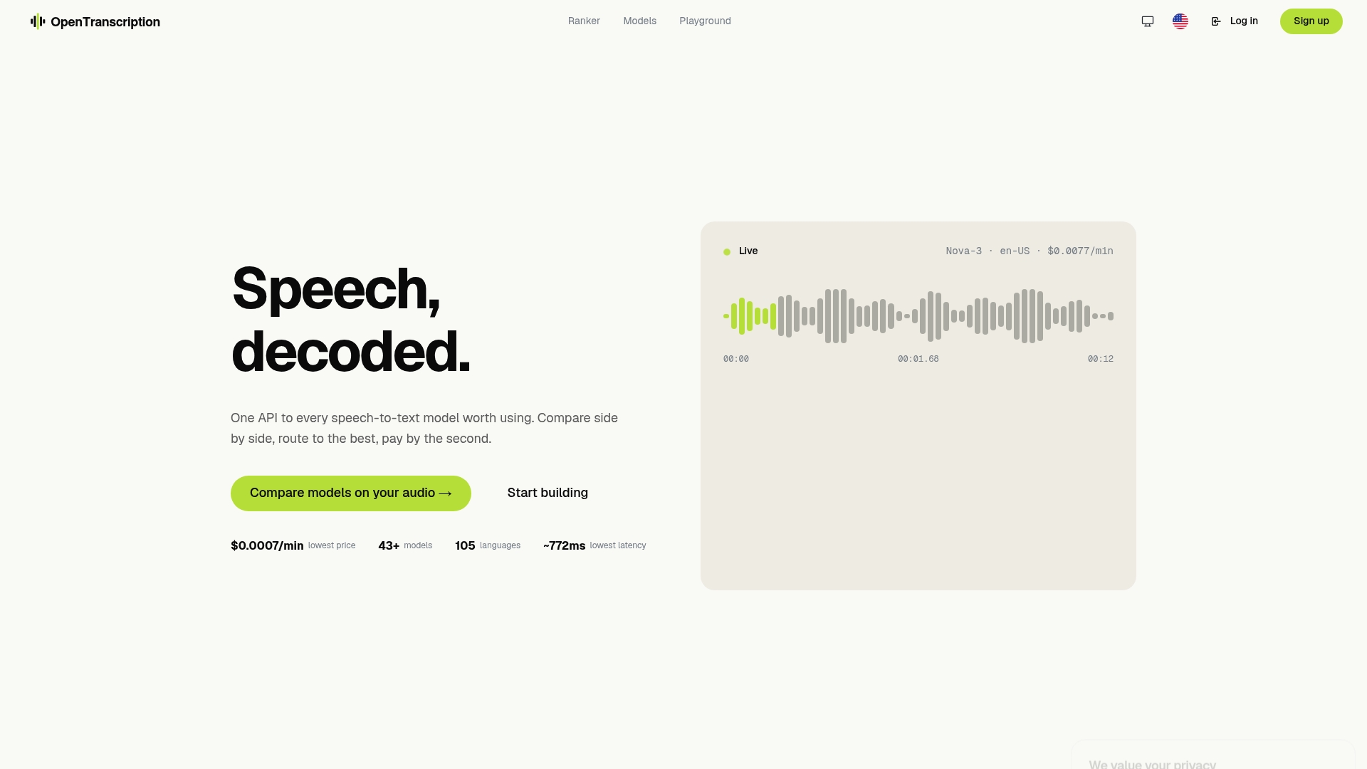
The platform’s model comparison and benchmarking interface lets engineers test multiple streaming models against their own audio in minutes, with side-by-side latency, accuracy, and cost data. Speaker identification, word-level timestamps, confidence scores, and support for 105+ languages are available across the model catalog. For teams evaluating whether to self-host or use a managed API, the realtime model rankings provide the benchmark data needed to make that decision without running a full internal evaluation suite. Sign up for an API key and run your first streaming diarization test against your own audio at opentranscription.io.

---

Useful sources and documentation to read next

The following references cover official documentation, open-source repositories, and research benchmarks that directly support the implementation patterns described in this guide.

• Real-time diarization quickstart — Microsoft Azure Speech Service: Official quickstart for the Conversation Transcriber API; shows how to access SpeakerId fields in real time and configure the managed streaming pipeline.
• Streaming with pyannote.ai: Documents the 100ms chunk protocol, the 5s server buffer limit, and the end_of_stream best practice; the primary reference for WebSocket streaming implementation details.
• diart — juanmc2005/diart (GitHub): Reference implementation for rolling-buffer incremental clustering with cannot-link constraints; includes latency configuration examples from 500ms to 5s.
• pyannote.audio (GitHub): The core open-source diarization library; hosts pretrained pipelines and documents GPU requirements and model hub access.
• Benchmarking Diarization Models — arXiv: Covers Sortformer v2 and related architectures; reports RTF benchmarks and missed-speech analysis across model families.
• Best Open-Source Speaker Diarization Models — Neosophie Blog: Comparative evaluation of NeMo, pyannote, and other open-source models; includes preprocessing effect analysis across model families.
• Streaming diarization documentation — Fluid Inference: Quantifies the 10–15% DER penalty for streaming vs. offline and explains the architectural reasons for the gap.
• azure-cognitiveservices-speech — PyPI: Python SDK for Azure Speech Service; installation reference for managed streaming integration.
• Python 3.10+ downloads: Runtime prerequisite for all open-source pipeline examples in this guide.
• OpenTranscription realtime model rankings: Side-by-side latency, accuracy, and cost benchmarks for streaming-capable models; useful for selecting a model without running an internal benchmark suite.
• OpenTranscription model catalog: Full catalog of supported transcription models with feature and trade-off profiles for streaming diarization use cases.

Recommended

• Scribe v2 Realtime: ElevenLabs makes its play for live speech-to-text · Signal
• Scribe v2 Realtime: model profile · Signal
• Deepgram Base: model profile · Signal
• Deepgram Enhanced: model profile · Signal

Article generated by BabyLoveGrowth