

Speaker Change Detection: A Technical Guide for Researchers and Developers
For most production pipelines, the fastest path to reliable speaker change detection (SCD) is SSL feature extraction with a lightweight classifier and contrastive pretraining — use wav2vec 2.0 or WavLM frozen features with a Bi-LSTM or small transformer head as your quick-start baseline. When your pipeline already includes an ASR encoder, the stronger choice is a joint ASR+SID+SCD model using the Continuous Integrate-and-Fire (CIF) mechanism, which produces token-aligned boundaries and outperforms frame-level detectors by 2.45% ECP on AISHELL-4. Evaluate everything with pyannote.metrics using a fixed tolerance collar and segment-wise purity/coverage alongside DER to keep comparisons reproducible.
Two practical starting recipes:
- Quick baseline: Extract frozen WavLM or wav2vec 2.0 features, compute cosine distance between adjacent segment embeddings, apply a tuned threshold, and score with pyannote.metrics ECP.
- Reproducible research baseline: Train a joint CIF-based ASR+SID+SCD model on AISHELL-4 or AMI, report token-boundary ECP and DER, and log all random seeds and dataset splits.
Pro Tip: Before committing to a full SSL fine-tuning run, verify your boundary label density. If your corpus has fewer than one speaker change per 10 seconds on average, class imbalance will dominate your loss and a focal loss or contrastive objective is not optional — it is a prerequisite.
Key Takeaways
| Point | Details |
|---|---|
| Start with SSL embeddings | Use frozen WavLM or wav2vec 2.0 features with a threshold or lightweight classifier as your first reproducible baseline. |
| Token-level CIF for ASR pipelines | Joint ASR+SID+SCD with CIF achieves 2.45% ECP improvement over frame-level detection on AISHELL-4. |
| Fix your evaluation protocol | Report collar value, overlap-exclusion rule, and pyannote.metrics version to make results reproducible and comparable. |
| MFCC for classical baselines | MFCCs outperform mel-spectrograms in BIC-GMM and KL-GMM unsupervised SCD experiments. |
| OpenTranscription for benchmarking | The model catalog and realtime rankings let you compare SSL and ASR backbones by accuracy, latency, and cost before committing to fine-tuning. |
Table of Contents
- What is speaker change detection and where does it fit in the audio pipeline?
- How to evaluate speaker change detection accurately
- Which datasets should you use for SCD experiments?
- Classical and embedding-based methods for detecting speaker changes
- State-of-the-art SCD with SSL models and token-level CIF
- Practical pipeline checklist and common implementation pitfalls
- Open-source code and reproducible SCD experiments
- What are the hardest open problems in speaker change detection?
- A pragmatic view on deploying SCD in production
- OpenTranscription gives you a benchmarked starting point for SCD-enabled transcription
- Sources
- FAQ
What is speaker change detection and where does it fit in the audio pipeline?
Speaker change detection is the task of identifying the precise timestamps in an audio stream where the active speaker transitions from one person to another. It is a binary boundary-detection problem: for each candidate time point, the system predicts whether a speaker change occurred. This distinguishes it from speaker diarization, which additionally assigns a speaker identity label to each segment, and from speaker segmentation, which groups audio into homogeneous speaker regions without necessarily locating the exact transition boundary.
In a standard multi-speaker audio pipeline, SCD occupies a specific slot:
- Voice Activity Detection (VAD): Removes non-speech regions and produces speech segments.
- Speaker change detection / segmentation: Subdivides speech segments at speaker-transition boundaries.
- Embedding extraction: Computes speaker embeddings (x-vectors, d-vectors, or SSL-derived representations) per sub-segment.
- Clustering / diarization: Groups sub-segments by speaker identity.
- Optional supervised identification or ASR alignment: Maps clusters to named speakers or aligns boundaries with ASR word timestamps.
SCD errors propagate directly into diarization: a missed boundary merges two speakers into one segment, inflating the DER metric, while a false alarm splits a single-speaker segment and adds spurious embedding comparisons. Getting SCD right is therefore a prerequisite for accurate automated speaker identification downstream.
Token-level SCD, where boundaries are predicted at ASR token positions rather than at fixed frame intervals, is the preferred approach when an ASR encoder is already in the pipeline. It reduces the candidate boundary rate, which lowers inference cost, and aligns naturally with word-level transcript segmentation. Frame-level or embedding-based SCD remains the practical choice when no ASR component is present or when latency constraints preclude a full encoder pass.
Pro Tip: If your VAD is aggressive and merges short pauses between speakers, SCD will systematically miss boundaries at those junctions. Run a boundary-density audit on your VAD output before training any SCD model — a merged pause looks identical to a mid-speaker pause and will silently corrupt your labels.
How to evaluate speaker change detection accurately
Reproducible evaluation is the single most common failure point in published SCD work. Tolerance collar choice, overlap handling, and metric selection all interact in ways that make cross-paper comparisons unreliable unless the protocol is stated explicitly.
- Precision, recall, and F1 for boundary detection: A predicted boundary is a true positive if it falls within a tolerance collar (typically 0.25 s or 0.5 s) of a reference boundary. Precision measures the fraction of predicted boundaries that are correct; recall measures the fraction of reference boundaries that are found. F1 is the harmonic mean. Collar choice has a large practical effect: widening from 0.25 s to 0.5 s can shift F1 by several absolute points on meeting corpora, which is why pyannote.metrics warns explicitly about tolerance parameter mismatches across studies.
- Segment-wise purity and coverage: Purity measures how homogeneous each predicted segment is with respect to reference speakers; coverage measures how well reference speaker regions are covered by predicted segments. These are more informative than boundary F1 alone when segment duration varies widely.
- Diarization Error Rate (DER): The DER metric sums missed speech, false alarm speech, and speaker confusion errors as a fraction of total reference speech duration. It is the standard summary metric for downstream diarization quality and reflects SCD errors indirectly through their effect on clustering.
- Equal Coverage-Purity (ECP): ECP is the operating point where purity equals coverage on the purity-coverage curve, analogous to the equal error rate in verification. It is the preferred single-number summary for SCD-specific evaluation because it is threshold-independent.
- Word Diarization Error Rate (WDER): When SCD feeds an ASR pipeline, WDER measures diarization errors at the word level and is the most task-relevant metric for transcription applications.
Statistic callout: Changing the tolerance collar from 0.25 s to 0.5 s can shift boundary F1 by several absolute percentage points on meeting corpora — a difference large enough to reverse the ranking of two competing systems if they are not evaluated under identical conditions.
Pro Tip: Always report the exact collar value, whether overlapping speech regions are excluded from scoring, and the pyannote.metrics version used. Without these three parameters, your numbers cannot be reproduced or fairly compared with prior work.
Which datasets should you use for SCD experiments?
Choosing the right corpus depends on whether you need controlled conditions for method development or realistic noise for generalization testing.
| Dataset | Domain | Speakers/Session | Annotation Type | Best Use |
|---|---|---|---|---|
| AMI | Meeting (English) | 4 per session | Manual segment + word alignment | Controlled multi-speaker baseline |
| ICSI | Meeting (English) | 6–9 per session | Manual segment labels | Noisier meeting conditions |
| CALLHOME | Telephone (multi-lang) | 2–7 | Manual segment labels | Conversational, channel noise |
| AISHELL-4 | Meeting (Mandarin) | 4–8 | Manual + forced alignment | Token-level SCD; CIF experiments |
| VoxConverse | Broadcast/wild (English) | Variable | Manual diarization labels | Domain mismatch, real-world noise |
The AMI Meeting Corpus provides both manual transcripts and forced-alignment word boundaries, making it the standard choice for controlled SCD experiments where you need reproducible train/dev/test splits. AISHELL-4 is the preferred corpus for token-level CIF experiments because its annotation supports forced-alignment boundaries that map directly to ASR token positions.
Key considerations when selecting a corpus:
- AMI and ICSI provide manual segment labels but vary in microphone array quality; use the individual headset microphone (IHM) condition for clean baselines and the array microphone (MDM) condition for noise robustness tests.
- CALLHOME is valuable for telephone-channel generalization but lacks word-level alignment in most releases, limiting its use for token-level SCD training.
- VoxConverse and DIHARD-style corpora are appropriate for final generalization evaluation but are too heterogeneous for controlled ablation studies.
- For low-resource language experiments, AISHELL-4 provides a non-English meeting corpus with sufficient annotation quality for token-level training.
Classical and embedding-based methods for detecting speaker changes
Classical SCD methods remain useful as fast, interpretable baselines and are often competitive on clean, close-microphone data. The two dominant unsupervised approaches are BIC-GMM (Bayesian Information Criterion with Gaussian Mixture Models) and KL-GMM (KL-divergence between adjacent window GMMs). Both segment audio into short windows, fit a GMM to each window’s acoustic features, and declare a boundary when the distance between adjacent models exceeds a threshold.
Feature choice matters substantially in these setups. Empirical comparisons show MFCCs consistently outperform mel-spectrograms across both BIC-GMM and KL-GMM baselines, with mel-spectrograms ranking lowest in the tested configurations. Zero-crossing rate and pitch features add marginal value in clean speech but degrade under noise.
Embedding-based methods replace GMM distance with speaker embedding distance. The standard approach computes x-vectors or d-vectors for adjacent fixed-length windows and scores cosine distance against a threshold. Siamese network architectures extend this by training a pairwise classifier directly on embedding pairs, which improves calibration but requires labeled change/no-change pairs for training.
SincNet, a CNN architecture that learns sinc-function-based filters directly from raw waveforms, serves as an effective supervised SCD encoder. Paired with a Bi-LSTM classifier head, it produces competitive frame-level SCD without requiring hand-crafted features. The HHousen speaker-change-detection GitHub repository provides a reference implementation of embedding-based SCD with configurable encoder backbones, including SincNet variants, and is a practical starting point for supervised baselines.
Key implementation notes for classical and embedding-based methods:
- Use pyannote.audio’s segmentation pipeline as a reference baseline; it implements embedding-difference SCD with configurable backbones and is directly compatible with pyannote.metrics scoring.
- Threshold calibration on a held-out development set is critical. A threshold tuned on training data will overfit to in-domain silence patterns and fail on new recording conditions.
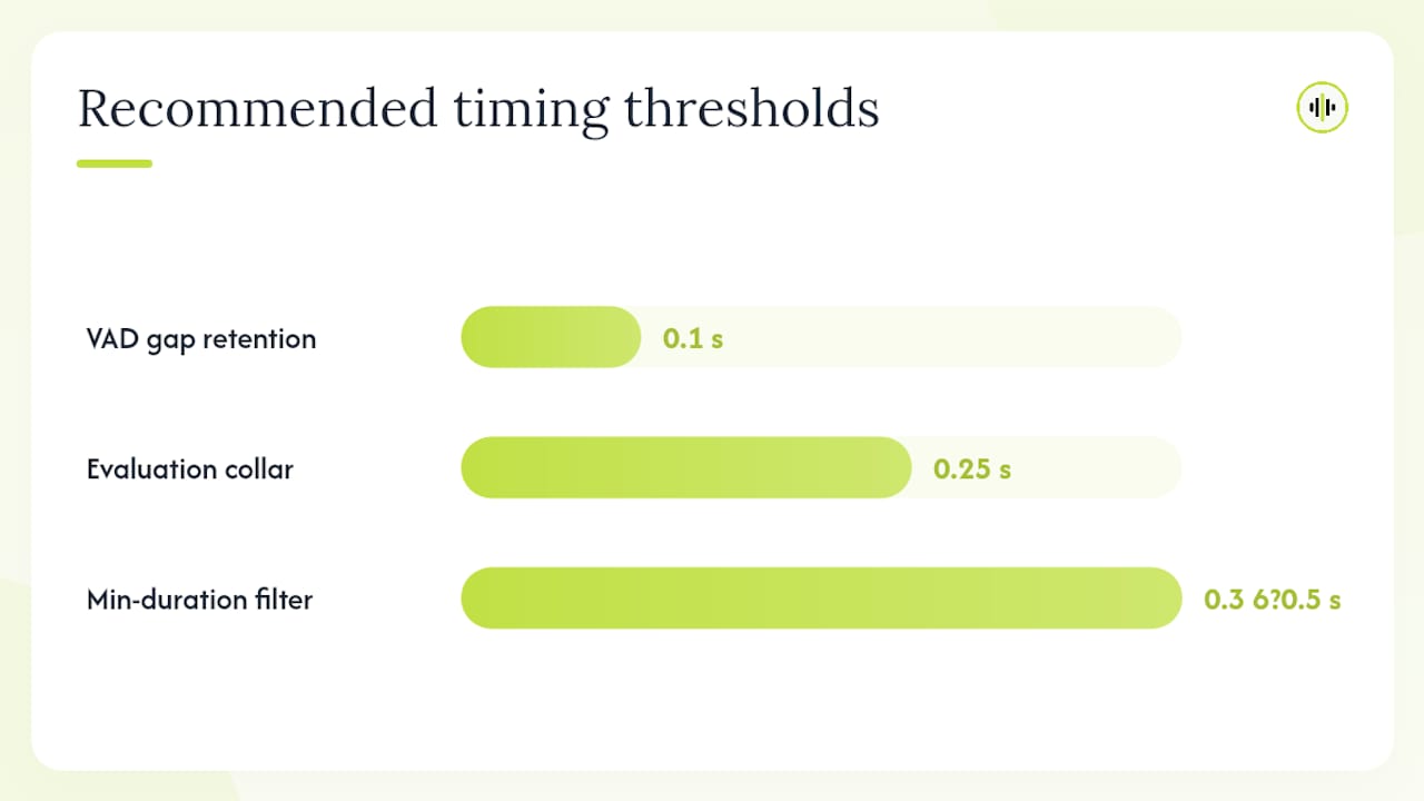
- Post-processing with a minimum-duration constraint (typically 0.3–0.5 s) suppresses spurious boundaries caused by brief acoustic events.
Pro Tip: When calibrating thresholds for embedding-based SCD, plot the full precision-recall curve on your dev set rather than optimizing a single operating point. The shape of the curve reveals whether your embedding space is well-separated — a flat curve with no clear knee indicates the embedding model needs fine-tuning before threshold tuning will help.
| Method | Feature | Supervision | Compute | Typical Strength |
|---|---|---|---|---|
| BIC-GMM / KL-GMM | MFCC | None | Very low | Fast unsupervised baseline |
| x-vector / d-vector distance | Speaker embeddings | Minimal | Low | Good on clean, close-mic data |
| SincNet + Bi-LSTM | Raw waveform | Supervised | Medium | Competitive supervised baseline |
| Siamese pairwise classifier | Any embedding | Supervised | Medium | Better calibration than threshold |
State-of-the-art SCD with SSL models and token-level CIF
Self-supervised learning models — wav2vec 2.0, WavLM, and HuBERT — currently set the strongest SCD benchmarks across most corpora. Their representations encode both acoustic and speaker-discriminative information at a level that classical features cannot match. However, SSL models require substantial labeled data and compute to fine-tune effectively, and contrastive learning is a key strategy for reducing overfitting risk when SCD labels are sparse.
The token-level CIF approach, introduced in Fan et al. (Interspeech 2022), addresses a fundamental limitation of frame-level SCD: frame boundaries are arbitrary with respect to linguistic structure, which means the model must learn to ignore within-phoneme variation while detecting between-speaker variation. CIF (Continuous Integrate-and-Fire) accumulates acoustic energy and fires a token boundary when a threshold is reached, producing token-aligned acoustic segments. A joint ASR+SID+SCD model trained with CIF then computes speaker-difference embeddings between adjacent tokens rather than adjacent frames. Token-level speaker-difference signals outperform frame-level differences in ablation experiments, and the joint model achieves a 2.45% ECP improvement over a frame-level baseline on AISHELL-4.
Multi-modal SCD, which combines audio embeddings with ASR-derived text embeddings and applies focal loss for class imbalance, further improves detection accuracy. Fine-tuning pre-trained models yields substantially better results than freezing them.
| Approach | Candidate Rate | Compute | Annotation Needs | Typical Gain vs. Baseline |
|---|---|---|---|---|
| Frame-level SSL classifier | High (every frame) | High | Segment labels | Strong |
| Embedding-difference (SSL features) | Medium (windowed) | Medium | Segment labels | Moderate |
| Token-level CIF (joint ASR+SCD) | Low (token rate) | Medium-high | Word/token alignment | Strongest (2.45% ECP on AISHELL-4) |
| Multi-modal (audio + text) | Medium | High | Segment + transcript | Strong, especially on meetings |
Two actionable recipes:
- Recipe A — SSL feature + contrastive pretraining: Fine-tune WavLM or wav2vec 2.0 with a contrastive loss on speaker-change/no-change pairs, then attach a lightweight classifier head. Use focal loss to handle the class imbalance between change and non-change frames.
- Recipe B — Joint ASR+SID+SCD with CIF: Train a CIF-based encoder jointly on ASR, speaker identification, and SCD objectives. Use AISHELL-4 or AMI IHM as the primary training corpus. Report token-boundary ECP and DER.
Ensemble and transformer-transducer augmentations represent an active research direction. Ensemble prediction approaches and transformer-transducer augmentations have both shown improvements in hybrid architectures, particularly for streaming SCD where token-level losses align naturally with the transducer’s sequential output.
Pro Tip: When fine-tuning WavLM or HuBERT for SCD, freeze the first 6 transformer layers and fine-tune only the upper layers and the classification head for the first 5 epochs. This prevents catastrophic forgetting of the low-level acoustic representations that make SSL features valuable for SCD in the first place.
Practical pipeline checklist and common implementation pitfalls
Building a production-ready SCD system requires more than a well-trained model. The following checklist covers the full pipeline from audio preparation to deployment.
- Audio preparation: Resample all audio to 16 kHz mono. Apply VAD to remove non-speech and verify that VAD output preserves short inter-speaker pauses (minimum 0.1 s gap retention recommended).
- Feature extraction: For classical methods, extract 13–40 MFCC coefficients with delta and delta-delta. For SSL methods, extract features from the target transformer layer (layer 6–9 for WavLM tends to be most speaker-discriminative).
- Model selection: Start with embedding-difference SCD for fast prototyping. Move to token-level CIF when ASR integration is required or when boundary precision is the primary constraint.
- Thresholding: Tune on a held-out development set using ECP as the operating criterion. Never tune on the test set.
- Post-processing: Apply a minimum-duration filter (0.3–0.5 s) to suppress spurious boundaries. Apply a merge rule to collapse boundaries separated by less than the minimum segment duration.
- Evaluation: Score with pyannote.metrics using a fixed 0.25 s collar, excluding overlapping speech regions from boundary scoring unless overlap handling is explicitly part of the system.
Annotation and labeling considerations:
- Use forced alignment to generate token-level boundaries from existing transcripts rather than manual boundary annotation where possible.
- For data augmentation, generate synthetic speaker-change boundaries by concatenating utterances from different speakers with realistic silence durations drawn from your target domain.
- Label overlapping speech regions explicitly and decide upfront whether your SCD system is expected to detect boundaries within overlapping turns.
Common pitfalls that waste significant engineering time:
- Protocol mismatch: Evaluating with a different collar or overlap-exclusion rule than prior work makes your numbers incomparable. Fix the protocol before running any experiments.
- In-domain silence overfitting: Models trained on one recording environment learn to use silence duration as a proxy for speaker change. This fails immediately on data with different inter-speaker pause distributions.
- Overlap blindness: Most SCD models are trained on clean single-speaker segments and produce undefined behavior on overlapping speech. If your target domain has overlap rates above 5%, add overlap-aware training data.
- Embedding drift: Speaker characteristics shift over long recordings (fatigue, emotion, microphone movement). A fixed threshold calibrated on short segments will accumulate false alarms over 30+ minute recordings.
Pro Tip: *Run a boundary density sanity check before training: compute the average number of reference boundaries per minute across your training set.
Open-source code and reproducible SCD experiments
The minimal toolkit for reproducible SCD experiments consists of three components: a feature extraction and modeling library, a metrics library, and a reference implementation to validate against.
Key toolkits and repositories:
- pyannote.audio: Provides end-to-end segmentation and diarization pipelines, pre-trained models, and training scripts. The segmentation model is the standard reference baseline for SCD on AMI and AISHELL-4.
- pyannote.metrics: Implements DER, segment-wise purity/coverage, ECP, and boundary precision/recall with configurable tolerance collars. The reference documentation covers both greedy and Hungarian mapping for DER computation — use greedy mapping for fast diagnostics and Hungarian for final reported numbers.
- SCDNet (arXiv): A dedicated SCD architecture with a published arXiv paper and associated training code; provides a clean baseline for comparing embedding-based and SSL-based approaches.
- HHousen speaker-change-detection: A GitHub repository with configurable encoder backbones (SincNet, x-vector, d-vector variants) and training scripts for supervised SCD.
- Fan et al. CIF repository: The token-level CIF ASR+SID+SCD codebase associated with the Interspeech 2022 paper; use this for reproducing token-boundary ECP results on AISHELL-4.
A minimal reproducible experiment on AMI IHM:
- Clone pyannote.audio and install dependencies (
pip install pyannote.audio). - Download AMI IHM using the official split from the AMI corpus page.
- Configure the segmentation model with a WavLM or wav2vec 2.0 backbone, 16 kHz input, and a 0.25 s minimum segment duration.
- Train with the standard AMI train split, validate on dev, and report on test.
- Score with
pyannote.metricsusingpython -m pyannote.metrics.segmentation --collar 0.25 --reference ref.rttm --hypothesis hyp.rttm. - Report ECP, DER, and boundary F1 at the 0.25 s collar. Log random seed, framework version, and dataset split hash.
Pro Tip: Pin your random seed, pyannote.audio version, and dataset split file checksums in a config.yaml at the start of every experiment. A single library update can shift DER by 0.5–1.0 absolute points through changes in VAD pre-processing alone — version pinning is the difference between a reproducible result and an unreproducible one.
What are the hardest open problems in speaker change detection?
Several challenges remain genuinely unsolved and represent active research directions worth pursuing.
- Overlapping speech: Most SCD models treat overlap as noise. Detecting speaker changes within overlapping turns requires either multi-channel input or a dedicated overlap-aware architecture. Current models trained on single-speaker segments produce inconsistent outputs when two speakers talk simultaneously.
- Low-resource languages and domain mismatch: SSL models pretrained on English-dominant corpora transfer poorly to tonal languages, accented speech, and non-meeting domains. Domain-adaptive fine-tuning with as few as 10–20 hours of target-domain data can recover significant performance, but the optimal adaptation strategy (full fine-tuning vs. adapter layers vs. prompt tuning) remains an open question.
- Real-time latency constraints: Token-level CIF models require a full encoder pass before firing boundaries, which introduces latency proportional to the token duration. Transformer-transducer augmentations offer a path to streaming SCD with bounded latency, but the accuracy-latency trade-off is not yet well characterized across domains.
- Evaluation standardization: The field lacks a single agreed-upon evaluation protocol. Different papers use different collars, different overlap-exclusion rules, and different DER implementations, making cross-paper comparisons unreliable without re-running all systems under a common protocol.
- Reliable boundary labeling for overlapping turns: Annotating the exact onset of a speaker change within an overlapping segment is subjective and inter-annotator agreement is typically lower than for clean turn-taking. This label noise propagates into model training and evaluation.
Promising research directions include multi-modal SCD (audio + ASR text + visual cues for video conferencing), self-supervised pretraining objectives tailored specifically for boundary detection rather than speaker verification, attention entropy analysis as a proxy for speaker-change probability in transformer models, and evaluation metrics that are insensitive to the specific tolerance collar choice.
Pro Tip: For low-resource adaptation, contrastive learning on unlabeled target-domain audio — without any SCD labels — can substantially improve the speaker-discriminative quality of SSL features before you add any supervised fine-tuning. This two-stage approach (unsupervised domain adaptation, then supervised SCD fine-tuning) consistently outperforms direct fine-tuning on small labeled sets.
A pragmatic view on deploying SCD in production
The gap between published SCD results and production performance is wider than most papers acknowledge. Benchmark numbers on AMI IHM or AISHELL-4 are measured under controlled conditions with clean annotation, fixed microphone setups, and known speaker counts. Production audio arrives with variable recording quality, unknown speaker counts, overlapping speech, and domain shift that no training corpus fully anticipates.
The practical recommendation is to start with embedding-based SCD using frozen SSL features. It is fast to deploy, requires no ASR infrastructure, and its failure modes are predictable: it struggles with very short turns and with speakers whose voices are acoustically similar. These failure modes are diagnosable from the precision-recall curve shape, which makes debugging tractable.
Move to token-level CIF-based SCD only when ASR is already integrated into the pipeline and when boundary precision at the word level is a hard requirement. For latency-sensitive streaming applications, the transformer-transducer augmentation path is worth evaluating before committing to a full CIF architecture.
The most underappreciated production pitfall is evaluation protocol drift: a system tuned and evaluated with a 0.5 s collar will appear to perform well in development but will produce noticeably more fragmented transcripts in production, where users perceive boundaries at a finer granularity. Aligning your evaluation collar with the granularity your downstream application actually requires is not a methodological nicety — it is the only way to know whether your system is production-ready.
Transparent benchmarking across multiple models, as OpenTranscription provides through its model catalog, is the most reliable way to identify which ASR and SSL backbone gives the best accuracy-latency trade-off for a specific domain before committing to a fine-tuning run.
OpenTranscription gives you a benchmarked starting point for SCD-enabled transcription
Selecting the right model backbone for speaker change detection is faster when you can compare accuracy, latency, and cost across a live catalog rather than running each candidate from scratch. OpenTranscription’s model catalog covers 40+ transcription models with structured profiles that include word-level timestamps, confidence scores, and speaker diarization support — the exact outputs SCD pipelines consume downstream.
For teams evaluating SSL backbones or ASR-integrated SCD architectures, the realtime model rankings surface latency-optimized models that are compatible with streaming SCD deployments. Pay-as-you-go billing with no subscription means you can run comparative benchmarks across multiple candidate models without committing to a long-term contract. Browse the model catalog or run a benchmark on your own audio at Opentranscription.
Sources
The following papers and toolkits are the core references for reproducing the experiments and evaluation protocols described in this article. Cite them when reporting SCD results.
- pyannote.metrics: reproducible evaluation for speaker diarization (Bredin et al., Interspeech 2017)
- Comparative Analysis of Audio Features for Unsupervised Speaker Change Detection (MDPI)
FAQ
What is speaker change detection and how does it differ from diarization?
Speaker change detection identifies the timestamps where one speaker transitions to another, producing a binary boundary signal. Speaker diarization goes further by assigning a speaker identity label to each resulting segment.
Which metric should you use to evaluate SCD systems?
Equal Coverage-Purity (ECP) is the preferred threshold-independent metric for SCD-specific evaluation; report it alongside DER and boundary F1 at a fixed 0.25 s collar using pyannote.metrics for reproducible comparisons.
When should you use token-level CIF SCD instead of frame-level methods?
Use token-level CIF when an ASR encoder is already in the pipeline and word-level boundary precision is required.
What is the best feature for classical unsupervised SCD baselines?
MFCCs consistently outperform mel-spectrograms in BIC-GMM and KL-GMM unsupervised SCD experiments, making them the recommended starting feature for classical baselines.
How does OpenTranscription support SCD experiments?
OpenTranscription’s model catalog and realtime rankings let you compare 40+ ASR and SSL-backed transcription models by accuracy, latency, and cost, giving you a benchmarked starting point for selecting SCD-compatible backbones without running each candidate from scratch.